Natural Science
Vol.11 No.01(2019), Article ID:90153,9 pages
10.4236/ns.2019.111005
Q Learning with Quantum Neural Networks
Wei Hu1, James Hu2
1Department of Computer Science, Houghton College, Houghton, NY, USA; 2Department of Computer and Information Science, University of Pennsylvania, Philadelphia, PA, USA
Correspondence to: Wei Hu, 
Copyright © 2019 by authors and Scientific Research Publishing Inc.
This work is licensed under the Creative Commons Attribution International License (CC BY 4.0).
http://creativecommons.org/licenses/by/4.0/


Received: January 2, 2019 ; Accepted: January 21, 2019 ; Published: January 24, 2019
ABSTRACT
Applying quantum computing techniques to machine learning has attracted widespread attention recently and quantum machine learning has become a hot research topic. There are three major categories of machine learning: supervised, unsupervised, and reinforcement learning (RL). However, quantum RL has made the least progress when compared to the other two areas. In this study, we implement the well-known RL algorithm Q learning with a quantum neural network and evaluate it in the grid world environment. RL is learning through interactions with the environment, with the aim of discovering a strategy to maximize the expected cumulative rewards. Problems in RL bring in unique challenges to the study with their sequential nature of learning, potentially long delayed reward signals, and large or infinite size of state and action spaces. This study extends our previous work on solving the contextual bandit problem using a quantum neural network, where the reward signals are immediate after each action.
Keywords:
Continuous-Variable Quantum Computers, Quantum Machine Learning, Quantum Reinforcement Learning, Q Learning, Grid World Environment

1. Introduction
Great success has been made in artificial intelligence, machine learning, deep learning, and reinforcement learning (RL). Deep learning based on neural networks has demonstrated its power in supervised learning problems such as computer vision and machine translation. On the other side, when applied to RL, amazing results like Alpha Go are possible. The goal of RL is to teach an agent to learn how to act from a given state in an unknown environment.
Different from the one-step decisions in supervised learning, the sequential decision making character in RL is observed in the process of the agent taking an action, and then receiving a reward and the next state, and then acting upon that state. The purpose of RL is for an agent to learn a strategy or policy that will obtain the maximum long-term cumulative rewards. In general, a policy is a distribution over actions given the states, which the agent uses to determine the next action based on the current state. The major RL algorithms are value based, policy gradient based methods, or a combination of both [1 - 3].
The development of machine learning today depends on three pillars: new algorithms, big data, and more powerful computers. To push current machine learning to a higher level of achievement, applying quantum computing to machine learning is an obvious and natural choice. A classical computer processes a classical bit of 0 or 1, while a digital quantum computer processes a qubit that can be in both states of 0 and 1 due to superposition. Furthermore, a continuous variable quantum computer can process a quantum state (one qumode) that can represent a complex number x + pi, where x is a superposition over all possible positions of a quantum particle and p is its super positioned momentum [4]. Two entangled quantum states are correlated with one another, meaning information on one quantum state will reveal information about the other unknown quantum state, which is much stronger than the correlation of classical data. When rolling two classical dice, the value of the second is independent of the value of the first, while when rolling two entangled quantum dice, the value of the second is determined by the value of the first. In the quantum case, we do not need to roll the second entangled quantum die once the value of the first is known.
When a quantum computer is utilized to solve a classical machine learning task, it typically requires the encoding of the classical data set into quantum states. Then, the quantum computer can process the quantum states and the result of the quantum computation is read by measuring the quantum system. Quantum computers can easily process quantum states that could correspond to vectors in very high-dimensional or even infinite-dimensional vector spaces, a task which is typically described as the curse of dimensionality in classical machine learning. With the current state of quantum computers, hybrid quantum-classical models are very popular. One well-known method is the variational approach to design quantum circuits with free parameters that can be optimized by both classical and quantum devices for a given machine learning objective. Therefore, the ability to compute gradients of variational quantum circuits is essential for this technique [5].
In the domain of quantum machine learning, RL has received relatively less attention, considering the quantum enhancements in supervised and unsupervised learning [6 - 18]. In our previous work [19], we solved the contextual bandit problem with a quantum neural network. Our current work is an extension to [19] by implementing the well-known RL algorithm Q learning using a quantum neural network. The Q learning algorithm learns a state-action value function that represents the value of taking action a when in state s. From the learned Q function, an optimal policy can be made.
2. Related Work
Because of the impressive performance of deep learning, creating neural networks on quantum computers has been a long-time effort [13 , 20 , 21]. The work in [22] proposed a general method to build a variational quantum circuit in a continuous-variable (CV) quantum architecture, composed of a layered structure of continuously parameterized photonic gates which can function like any classical neural network including convolutional, recurrent, and residual networks. Our current study uses the technique in [22] to design a quantum network to implement the Q learning algorithm.
The nonlinearity of the classical neural networks plays a key role in their success which is realized with a nonlinear activation function in each layer. In photonic quantum networks, this nonlinearity is accomplished with non-Gaussian photonic gates such as the cubic phase gate and the Kerr gate. The common representation of in the classical networks where f is the nonlinear activation function, W is the weight matrix and b is the bias can be emulated as layers of quantum gates in the CV model where D is an array of displacement gates, are interferometers, S are squeezing gates, and are non-Gaussian gates to have an effect of nonlinearity.
One quantum advantage of this type of quantum networks is that for certain problems, a classical neural network would take exponentially many resources to approximate the quantum network. It is shown in [22] that when a Fourier transform is applied to the first layer and last layer of a quantum network, which changes the input states from position states to momentum states and the position homodyne measurements to momentum ones. As we know, a momentum state can be represented as an equal superposition over all position states via Fourier transform. Therefore, this quantum circuit can be interpreted as acting on an equal superposition of all classical inputs, a task that would require exponentially many resources to replicate by a classical computer.
3. Methods
3.1. Grid World Environment
RL is characterized by the agent, the environment and their interaction. Therefore, each RL algorithm needs to be tested in certain environments. In this report, we use the grid world environment, which is a commonly adopted benchmark in RL. Compared with the contextual bandit problem studied in [19], the grid world is harder as it delays the positive reward until the goal state is reached. Grid world is a 2D rectangular grid, where an agent starts at one grid square (the start state) and tries to move to another grid square (the goal state). The goal of RL algorithms is for the agent to learn optimal paths on the grid to arrive at the goal state in the least number of steps. The agent can move in up, down, left, or right directions by one grid square. Our grid world is similar to the Frozen Lake environment from gym [https://gym.openai.com/envs/FrozenLake-v0/] but with a smaller 2 × 3 size while the standard size is 4 × 4. It is a 2 × 3 grid which contain four possible areas―Start (S), Frozen (F), Hole (H) and Goal (G) (Figure 1). The agent moves around the grid until it reaches the goal or the hole. If it falls into the hole, it has to start from the beginning and is rewarded the value 0. The process continues until it learns how to reach the goal eventually. The visual description of this grid world is in Figure 1.
The agent in this environment has four possible moves―up, down, left and right. The standard Frozen Lake environment has an option to allow moves to be slippery. If slippery, there could be a random move happening in every action since the agent is slipping in different directions on a frozen surface. The episode ends when the agent reaches the goal or falls in the hole. It receives a reward of 1 if it reaches the goal, and zero otherwise. There is a clear contrast between the contextual bandit problem [19] where the reward is immediate after each action and this grid world problem. In the grid world problem, the agent gets one reward signal at the end of a long episode of interaction with the environment, which makes it difficult to identify exactly which action was the good one.
3.2. Markov Decision Process
The aim of RL is to learn sequences of actions that will help an agent gain the maximum long-term rewards. Thus, the end product of RL is a strategy that tells an agent how to act from a particular state, and this strategy is usually named the policy in RL. The policy can be deterministic or stochastic. In the latter case, the policy produces a probability distribution over all the possible actions. In general, a policy is a mapping from states to actions.
The interaction of an agent and an environment in a typical RL problem can be formulated as a Markov decision process (MDP) [23]. It is a mathematical model of sequential decision making, which describes how actions in a certain state receive immediate rewards, but also the future rewards through subsequent states and actions. It is a framework used to formulate how to act in a stochastic environment. A
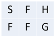
Figure 1. The grid world of size 2 × 3 used in this study. Each grid (state) is labeled with a letter which has the following meaning: Start (S), Frozen (F), Hole (H) and Goal (G). The state G has a reward of one and other states have a reward of zero. Each grid (state) is represented as an integer from 0 to 5, with the top row: 0, 1, 2 (left to right) and the bottom row: 3, 4, 5 (left to right).
discrete, finite-state MDP is defined by a tuple , specifying a set of states S and actions A, a transition probability p, a reward function R, and a discount factor . The Markov property of MDP indicates that the future state transitions depend only on the present state and not the whole history of events that precede it. The MDP describes how the environment works and the policy controls how the agent behaves. The hard part of RL is to learn how a current action will affect future rewards, which is commonly called the return.
The return defines the total discounted sum of the rewards received:
(1)
Equation (1) describes a discounted return and is the discount rate. It makes the immediate rewards more valuable than those in the future.
Another common concept in RL is the Q function that can be formulated as below:
where the expectation is taken over potentially random actions, transitions, and rewards. The randomness comes from the fact that the policy can be stochastic, the transition from one state to another can be probabilistic, and the rewards returned by the environment can be varied, delayed or affected by unknown factors. The state-action value function of under a policy π is the expected return starting from s, taking the action a, and thereafter following policy π. The optimal state-action value function is defined as . Given a MDP, an agent can learn an optimal policy via simulation of interactions with the model. In this regard, there are policy iteration and value iteration algorithms to find an optimal policy since the rewards and transition probability are known and there is no need to explore the environment [1]. Model-based algorithms tend to be data efficient, but when the state space is large this approach is not feasible. For example, building a model for the game Go is impossible due to the number of possible moves.
3.3. Q Learning
In general, there are two main approaches to RL: 1) to learn a policy using a given model or learn a model of the world from experience and then use planning with that learned model to discover a policy (model-based) and 2) to learn a policy directly or a value function from experience then define a policy from it indirectly (model-free). The policy gradient approach tries to learn a good policy directly while Q learning attempts to learn the value of first, then from this Q function, an optimal policy can be deduced. Q learning can learn the optimal policy even when actions are selected by a different policy including a random policy.
Q Learning [24 , 25] is a model-free RL method that estimates the long-term expected return of executing an action a in state s. Without a model or in an unknown environment, the agent has to learn from experience, using an iterative process. The estimated returns, known as Q values, can be learned iteratively and the updating rule of Q values can be described as:
(2)
where the max is taken over all the possible actions in state , is the discount factor, and is the learning rate. The updating formula in Equation (2) suggests that the formation of the Q function is executed by following a greedy policy. To address the challenge of delayed rewards in many RL problem, Equation (2) gives credit to the past actions through backpropagation of the final reward with a discount factor. Equation (2) is known as the Bellman equation and is a key tool in RL. In a simple problem when the state space is small and every state is known, Q function can be represented as a table with states as rows and actions as columns. However, in a problem with a large state space or unknown states, deep neural networks have to be used instead, in which the loss function is the mean squared error of the predicted Q value and the TD-target Q value.
Mathematically, is a combination of immediate reward with all future rewards. The learned state-action value function Q is an approximation to the optimal value function which can be used to find the optimal policy, independent of the policy being employed in the learning process. The goal of RL is to choose the best action for any given state, which means the actions have to be ranked and the Q values can be used for this purpose. In this sense, Q learning is an iterative process of learning how to rank the actions in a given state. Naturally, there is a tension between the exploitation of known rewards, and exploration to discover new actions that could lead to better rewards. The quantity in Equation (2) is usually named TD-target and TD-target- is TD-error. We can see that TD-target is the maximum possible Q value for the next state while is the predicted Q value for the current state.
However, it is not straightforward to apply Q learning to the continuous action space. When the environment has an infinite number of actions, it is more efficient to use policy-based methods than the value-based. Say in Q learning, the updating rule (Equation (2)) needs to compute the quantity which requires a full scan of the action space.
3.4. Quantum Neural Network Representation of Q Functions
For a problem with a small number of states and actions, tables could be used to represent the Q function efficiently, but for large sizes of state and action spaces they do not scale well. In this case, neural networks can be employed to approximate the Q function with Q ( s, a; θ ) parameterized by θ (Figure 2).
The objective of training this neural network is to tune the values of the parameter θ to reduce the gap between the TD-target and the Q value, which is called TD-error. This method highlights the fact that the implementation of Q learning makes use of supervised learning techniques and the training of the quantum network is done by both quantum and classical devices with help from Tensor flow and Strawberry field simulation [26]. The input to the network is the state and the output is a list of Q value for each action. Notice that the output of the network is Q values, not a policy. We can extract a greedy policy with respect to the Q values. A policy is a function for the agent to select actions given states.
The training of this network is similar to the backpropagation of error in supervised learning. However, ground-truth labels are provided in supervised learning. RL can only use the TD-target that can be varied, delayed or affected by unknown variables. In a sense, it is a moving target.
In the case of our grid world example, we use a one-layer network which takes the state encoded as an integer (0 - 5), and produces a vector of 4 Q values, one for each action (Figure 2). Our loss function is a sum-of-squares loss, where the difference between the current predicted Q values and the TD-target value is computed and the gradients are passed through the network.
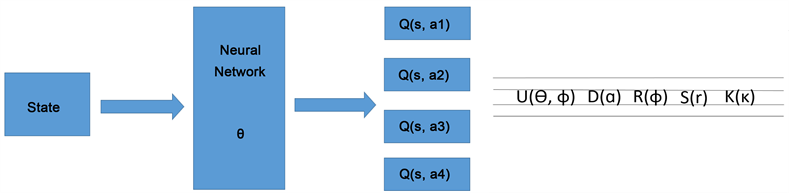
Figure 2. On the left, there is the logical representation of the network to compute the Q function (assuming there are 4 actions) and on the right, there is the physical representation of the actual parametrized circuit structure for a CV quantum neural network made of photonic gates: interferometer, displacement, rotation, squeeze, and Kerr (non-Gaussian) gates. The output is the Fock space measurements. More details of this quantum network can be found in [19 , 20].
4. Results
The grid world environment is widely used to evaluate RL algorithms. Our quantum Q learning is evaluated in this environment that is explained in Section 3.1. The aim of Q learning in this environment of size 2 × 3 is to discover a strategy that controls the behavior of an agent and helps to know how to act from a particular state. We run the algorithm in series of experiments, then take the average of the rewards and path lengths in each case, demonstrating that our quantum network is able to solve the grid world problem. In the non-slippery grid world, the optimal path length is 3, while in the slippery case, it takes more than 3 steps to arrive at the goal state G. One episode is defined as a sequence of moves from the start state S to a terminal state that can be either the hole H or the goal G in our grid world. Our results indicate that after about 5 episodes, the quantum network is able to learn how to reach the goal state G in three steps for the non-slippery case, but the learning in the slippery case is much harder (Figure 3).
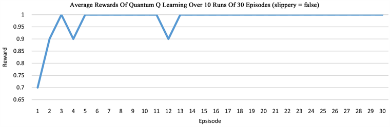
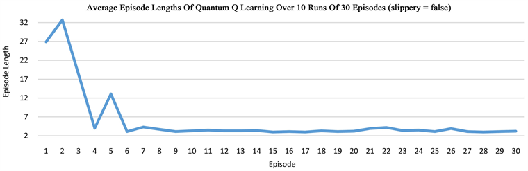
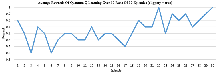
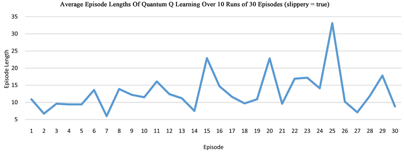

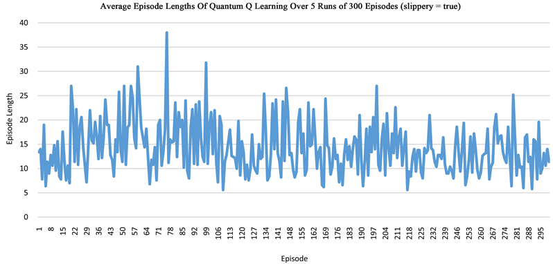
Figure 3. The plots show the learning of the quantum network in the grid world of size 2 × 3, measured by the average rewards or the episode length from state S to state G or state H.
5. Conclusion
In RL, there are model based and model free algorithms. The model based assumes that the agent has access to a model of the environment and learns from it while the model free assumes that the agent has no knowledge of a model and therefore must learn from direct experience with the environment. The Q learning that we use in this study is a model free algorithm.
Neural networks are widely used in deep learning, demonstrated as a great technique in supervised learning but can also be used in RL. As a famous RL algorithm, Q learning learns a Q function. The value of shows how favorable action a in state s is, measured by the long-term return. The updating rule of Q learning (Equation (2)) suggests that the value of an action depends on both the immediate reward and future rewards. In challenging RL problems, there are many states and actions, making it hard to store and ineffective to produce and update the Q values in a table, so a neural network is used to approximate the Q function.
It is trendy today to apply quantum computing to classical machine learning. In this report, we create a photonic quantum neural network to implement Q learning and test it in the grid world environment. The grid world problem is a more difficult task than the contextual bandit problem in [19], in which a reward is immediate after each action. Our findings indicate that the quantum network is able to solve the grid world problem and that the slippery grid world is harder to solve than the non-slippery one. The training of this quantum network is conducted by both quantum and classical devices, demonstrating the advantage of a hybrid approach.
The interest in developing quantum machine learning algorithms has been on the rise in recent years and their potential needs to be further explored. In this regard, our work provides another example of how to implement a classical RL algorithm using a quantum device, which extends our previous work on solving the contextual bandit problem using a quantum network.
Conflicts of Interest
The authors declare no conflicts of interest regarding the publication of this paper.
References
- 1. Sutton, R.S. and Barto, A.G. (2018) Reinforcement Learning: An Introduction. 2nd Edition, A Bradford Book, Cambridge, MA.
- 2. Ganger, M., Duryea, E. and Hu, W. (2016) Double Sarsa and Double Expected Sarsa with Shallow and Deep Learning. Journal of Data Analysis and Information Processing, 4, 159-176. https://doi.org/10.4236/jdaip.2016.44014
- 3. Duryea, E., Ganger, M. and Hu, W. (2016) Exploring Deep Reinforcement Learning with Multi Q-Learning. Intelligent Control and Automation, 7, 129-144. https://doi.org/10.4236/ica.2016.74012
- 4. Serafini, A. (2017) Quantum Continuous Variables: A Primer of Theoretical Methods. CRC Press, Boca Raton.
- 5. Peruzzo, A., McClean, J., Shadbolt, P., Yung, M.-H., Zhou, X.-Q., Love, P.J., Aspuru-Guzik, A. and O’Brien, J.L. (2014) A Variational Eigenvalue Solver on a Photonic Quantum Processor. Nature Communications, 5, Article No.: 4213. https://doi.org/10.1038/ncomms5213
- 6. Clausen, J. and Briegel, H.J. (2018) Quantum Machine Learning with Glow for Episodic Tasks and Decision Games. Physical Review A, 97, 022303. https://doi.org/10.1103/PhysRevA.97.022303
- 7. Crawford, D., Levit, A., Ghadermarzy, N., Oberoi, J.S. and Ronagh, Pooya (2016) Reinforcement Learning Using Quantum Boltzmann Machines. arXiv:1612.05695 [quant-ph].
- 8. Dunjko, V., Taylor, J.M. and Briegel, H.J. (2018) Advances in Quantum Reinforcement Learning. arXiv:1811.08676 [quant-ph].
- 9. Biamonte, J., Wittek, P., Pancotti, N., Rebentrost, P., Wiebe, N. and Lloyd, S. (2017) Quantum Machine Learning. Nature, 549, 195-202. https://doi.org/10.1038/nature23474
- 10. Dunjko, V. and Briegel, H.J. (2018) Machine Learning and Artificial Intelligence in the Quantum Domain: A Review of Recent Progress. Reports on Progress in Physics, 81, 074001. https://doi.org/10.1088/1361-6633/aab406
- 11. Hu, W. (2018) Empirical Analysis of a Quantum Classifier Implemented on IBM’s 5Q Quantum Computer. Journal of Quantum Information Science, 8, 1-11. https://doi.org/10.4236/jqis.2018.81001
- 12. Hu, W. (2018) Empirical Analysis of Decision Making of an AI Agent on IBM’s 5Q Quantum Computer. Natural Science, 10, 45-58. https://doi.org/10.4236/ns.2018.101004
- 13. Hu, W. (2018) Towards a Real Quantum Neuron. Natural Science, 10, 99-109. https://doi.org/10.4236/ns.2018.103011
- 14. Hu, W. (2018) Comparison of Two Quantum Clustering Algorithms. Natural Science, 10, 87-98. https://doi.org/10.4236/ns.2018.103010
- 15. Ganger, M. and Hu, W. (2019) Quantum Multiple Q-Learning. International Journal of Intelligence Science, 9, Article ID: 89926. https://doi.org/10.4236/ijis.2019.91001
- 16. Naruse, M., Berthel, M., Drezet, A., Huant, S., Aono, M., Hori, H. and Kim, S.-J. (2015) Single-Photon Decision Maker. Scientific Reports, 5, Article No. 13253. https://doi.org/10.1038/srep13253
- 17. Mitarai, K., Negoro, M., Kitagawa, M. and Fujii, K. (2018) Quantum Circuit Learning. arXiv:1803.00745
- 18. Schuld, M. and Killoran, N. (2018) Quantum Machine Learning in Feature Hilbert Spaces. arXiv:1803.07128
- 19. Hu, W. and Hu, J. (2019) Training a Quantum Neural Network to Solve the Contextual Multi-Armed Bandit Problem. Natural Science, 11, 17-27. https://doi.org/10.4236/ns.2019.111003
- 20. Farhi, E. and Neven, H. (2018) Classification with Quantum Neural Networks on Near Term Processors. arXiv:1802.06002
- 21. Dong, D., Chen, C., Li, H. and Tarn, T.-J. (2008) Quantum Reinforcement Learning. IEEE Transactions on Systems, Man, and Cybernetics, Part B (Cybernetics), 38, 1207-1220.
- 22. Killoran, N., Bromley, T.R., Arrazola, J.M., Schuld, M., Quesada, N. and Lloyd, S. (2018) Continuous-Variable Quantum Neural Networks. arXiv:1806.06871
- 23. Bellman, R. (1957) A Markovian Decision Process. Journal of Mathematics and Mechanics, 6, 679-684. https://doi.org/10.1512/iumj.1957.6.56038
- 24. Watkins, C.J. and Dayan, C.H. (1992) Technical Note: Q-Learning. Machine Learning, 8, 279-292. https://doi.org/10.1007/BF00992698
- 25. Watkins, C.J. (1989) Learning from Delayed Rewards. PhD Thesis, University of Cambridge, Cambridge.
- 26. Killoran, N., Izaac, J., Quesada, N., Bergholm, V., Amy, M. and Weedbrook, C. (2018) Strawberry Fields: A Software Platform for Photonic Quantum Computing. arXiv:1804.03159.