Natural Science
Vol.4 No.4(2012), Article ID:18627,12 pages DOI:10.4236/ns.2012.44034
Nature’s autonomous oscillators
![]()
1Applied Physics Laboratory, Johns Hopkins University, Laurel, USA; *Corresponding Author: hans.mayr@jhuapl.edu, hans.g.mayr@nasa.gov
2Goddard Space Flight Center, The National Aeronautics and Space Administration (NASA), Greenbelt, USA
35300 Thunder Hill Road, Columbia, Maryland, USA
4220 Chana Drive, Auburn, California, USA
Received 5 February 2012; revised 8 March 2012; accepted 20 March 2012
Keywords: Mechanical Clock; Quasi-biennial Oscillation; Bimonthly Oscillation; Solar Dynamo; Insect Flight; Human Heart
ABSTRACT
Nonlinearity is required to produce autonomous oscillations without external time dependent source, and an example is the pendulum clock. The escapement mechanism of the clock imparts an impulse for each swing direction, which keeps the pendulum oscillating at the resonance frequency. Among nature’s observed autonomous oscillators, examples are the quasi-biennial oscillation of the atmosphere and the 22- year solar oscillation [1]. Numerical models simulate the oscillations, and we discuss the nonlinearities that are involved. In biology, insects have flight muscles, which function autonomously with wing frequencies that far exceed the animals' neural capacity. The human heart also functions autonomously, and physiological arguments support the picture that the heart is a nonlinear oscillator.
1. INTRODUCTION
Among nature’s oscillators, the lunar tide is a wellunderstood familiar example. The sea level rises and falls with a period of about 12 hours, which is produced by the gravitational interaction of the moon circling the Earth. Another example is the diurnal atmospheric tide, which is produced by variable solar heating. Generated by external time dependent forcing, the tides are not autonomous oscillators. Oscillations that are forced by a time dependent source can be understood in terms of a linear system. Take n linear equations with n unknowns, A(n, n)·X(n) = S(n), A the square matrix of terms that account for dissipation, X the unknown linear column vector, and S the source vector. With X(n) = A−1(n, n)·S(n), A−1 the inverse matrix, it follows that an oscillation X ≠ 0 is produced with a source S ≠ 0 (Finite differencing produces the matrix elements for A to obtain a solution for a system of linear differential equations). In space physics, there is a large scientific body of literature featuring linear mathematical models that can generate and reproduce a variety of observed oscillations applying known excitation sources.
The above linear analysis demonstrates, with X(n) = A−1(n, n)·S(n), that for S = 0, X = 0. This means that without an external time dependent source, a linear system cannot produce an oscillation. Autonomous oscillators must be nonlinear—and a familiar example of such an oscillator is the pendulum clock. Once initiated, the clock continues oscillating at the resonance frequency that is determined by the length of the pendulum. The external source for the clock is the steady force of the weight pulling on the drive chain that activates the escapement wheel. With sufficient energy from the suspended weights to overcome friction, the escapement mechanism provides the impulse/nonlinearity that keeps the pendulum oscillating, as illustrated in Figure 1.
In mathematical terms, the variables (x, y) interact in a nonlinear system, like a1·xy + b1·xy = s1, a2·xy + b2·xy = s2, or for example a1·x2 + b1·y3 = s1, a2·x2 + b2·y3 = s2, where a12 and b12 account for dissipation such as friction, and s1, s2 are external sources that would be zero for the mechanical clock. A simple example of nonlinear interaction is illustrated with the temperature feedback of snow. In winter at high latitudes, as it gets colder, the precipitation turns into snow. White snowflakes, covering the ground, reflect incoming solar radiation to make it still colder. The interaction between diminishing radiation and resulting formation of ice crystals, two variables of climate change, say x, y, produce the nonlinear term, xy, that accelerates cooling. Another example of climate change is the melting of glaciers due to CO2-induced global warming. As the glaciers melt, the dark surface gets exposed and absorbs more solar radiation to acelerate the warming. Emptying a bottle with fluid would
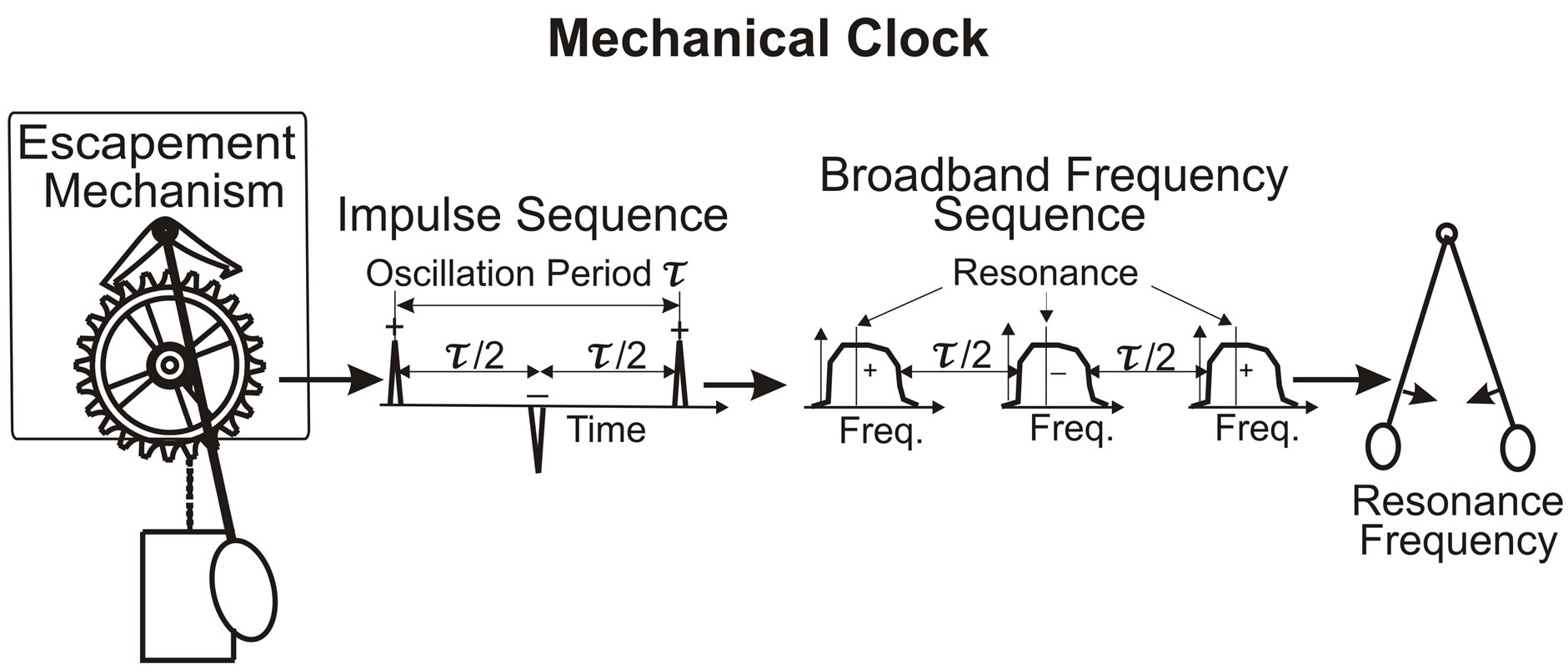
Figure 1. In the mechanical clock, the escapement mechanism produces the impulse/nonlinearity that generates the oscillation without external time dependent source. Illustrated are the impulse sequence and broadband frequency sequence, which produce the pendulum oscillation with resonance frequency.
be a hands-on experiment demonstrating a nonlinear oscillation. The fluid pouring out, with sufficient speed, is compressed in the bottleneck. The resulting increase in pressure caused by the flow, a nonlinear feedback, slows down the flow to produce a glugging oscillation.
[1] reviewed the properties of observed fluid dynamical autonomous oscillators in space physics, foremost the quasi-biennial oscillation in the Earth’s atmosphere with a period of about two years, and the 22-year oscillation of the solar dynamo magnetic field. The oscillations have been simulated in numerical models without external time dependent source, and in Section 2 we summarize the results. Specifically, we shall discuss the nonlinearities involved in generating the oscillations, and the processes that produce the periodicities.
Stretch-activation of muscle contraction is the mechanism that produces the high frequency oscillation of autonomous insect flight, briefly discussed in Section 3. The same mechanism is also invoked to explain the functioning of the cardiac muscle. In Section 4, we present a tutorial review of the cardio-vascular system, heart anatomy, and muscle cell physiology, leading up to Starling’s Law of the Heart, which supports our notion that the human heart is also a nonlinear oscillator. In Section 5, we offer a broad perspective of the tenuous links between the modeled fluid dynamical oscillators and the human heart physiology.
2. FLUID-DYNAMICAL OSCILLATORS
In space physics, like in other areas of environmental science, mathematical models have been widely used to provide a physical understanding of the observations. Mentioned in the introduction, a large number of phenomena can be understood in terms of linear systems, like the diurnal atmospheric tide that is produced by variable solar heating. But there is no such external time dependent source known, which could produce the observed quasi-biennial oscillation in the atmosphere or the 22-year oscillation of the solar magnetic field. Numerical models generate the oscillations through nonlinear interactions that produce periodicities determined by the internal dynamical properties of the fluids.
2.1. Quasi-Biennial Oscillation (QBO)
In the zonal circulation of the terrestrial stratosphere at low latitudes, the quasi-biennial oscillation (QBO) dominates, and [2] presented a comprehensive review of the observations and physical mechanisms that generate the oscillation. Observed with satellites and ground-based measurements, the wind velocities vary between eastward and westward regimes that propagate down and have periods averaging approximately 28 months. Since its discovery more than 40 years ago, research has shown that the QBO plays an important role in a multitude of processes that affect the climate, as in the transmission of solar activity signatures and modulation of atmospheric tides for example. In the spirit of the subject matter of the present paper, we consider the QBO isolated from interactions with other atmospheric oscillations and focus on the fundamental processes that generate the QBO.
In a seminal paper published in 1968, [3] demonstrated that the QBO can be generated with planetary waves, and their theory was confirmed in numerous modeling studies. Subsequent studies showed that the QBO could also be reproduced with parameterized gravity waves (GW) [4,5], and this is now well accepted [2]. [3] considered the QBO being driven by the 6-month semi-annual oscillation (SAO) generated by solar heating. But [6] subsequently concluded that the SAO was not essential for generating the QBO, and this was confirmed in a modeling study [7].
From that paper, we present in Figure 2 computer solutions produced with the Numerical Spectral Model [4,8], which incorporates the Doppler Spread Parameterization [9,10] that provides the GW momentum source and associated eddy diffusivity/viscosity. Applying factor of two different diffusion or dissipation rates, QBO-like oscillations are produced with periods of about 33 and 17 months (Figures 2(a) and (b), respectively), which differ in amplitude by about a factor of two. The numerical results were generated for perpetual equinox, without time dependent solar heating. Without external time dependent source, the excitation mechanism cannot be linear, as demonstrated in Section 1. A nonlinear process must be involved in generating the oscillations.
The nonlinearity is displayed in Figure 3, which shows the zonal winds, U, and the accompanying GW momentum source, MS, varying with altitude. Discussed by [1,7], the positive nonlinear feedback associated with critical level of wave absorption produces a MS with sharp peaks near vertical wind shears, dU/dr. Considering the wind oscillation of the QBO, varying with frequency ω, the nonlinear part of the MS, to first order, can
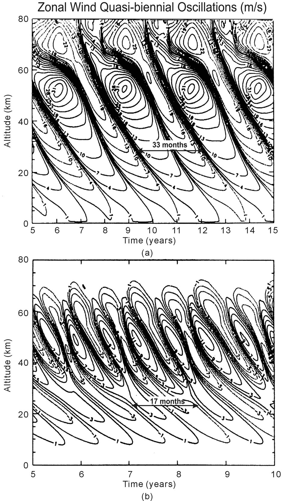
Figure 2. Altitude contour plots of equatorial zonal winds, positive eastward and negative westward. The winds were derived with diffusion/dissipation rates a factor of 2 larger in (b) than in (a). The resulting oscillation periods and amplitudes decrease with increasing dissipation rates; they are a factor of 2 smaller in (b) than in (a). A constant gravity wave (GW) flux provided the energy for the momentum source that generated the QBO-like oscillations. Figure taken from [7].
be written in the approximate form [dU(ω,r)/dr]3, of odd power. With complex notation, a source in the form [Exp(iωt)]3 produces the term with Exp[i(ω + ω + ω)t] for the higher order frequency, 3ω. Such a nonlinear source also generates Exp[i(ω + ω − ω)t] for the fundamental frequency ω, which maintains the oscillation.
2.2. Bimonthly Oscillation (BMO)
Zonal-mean oscillations with periods around 2 months have been seen in ground based and satellite wind measurements in the Earth atmosphere [12-14]. The Numerical Spectral Model generates such oscillations
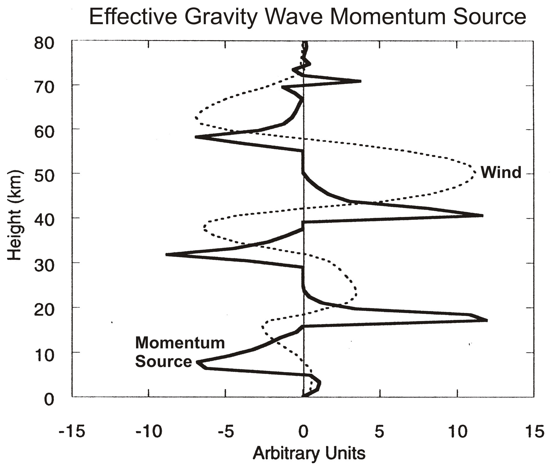
Figure 3. Snapshots are shown of zonal winds, and effective GW momentum source that generates the oscillations in Figure 2(b). The peak momentum source occurs near the maximum vertical velocity gradient; it varies in phase with the gradient and is strongly nonlinear. Figure taken from [11].
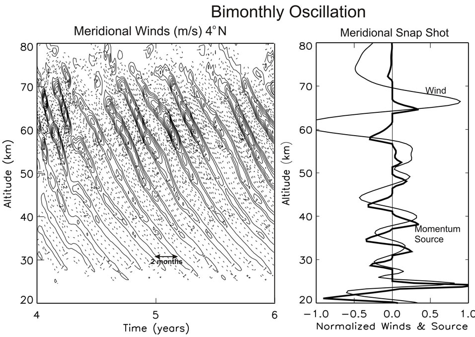
[15], and numerical experiments show that they are not produced when the gravity waves (GW) propagating north/south are turned off. In Figure 4(a), a computer solution is presented from that paper, which is produced only with the meridional (north/south) GW momentum source. Regular bimonthly oscillations (BMO) are generated with a period of about 2 months, which resemble the quasi-biennial oscillation (QBO) above discussed.
The similarity between the BMO and QBO is also evident in Figure 4(b), where meridional winds, V, are presented together with the associated momentum source. Like the GW source of the QBO in Figure 3, the momentum source in Figure 4(b) is sharply peaked near meridional wind shears. Discussed in Section 2.1, this impulsive momentum source can be viewed approximately as a nonlinear function of the velocity field, which has the character, [dV(ω,r)/dr]3. Such a non-linearity can generate an oscillation without external time-dependent forcing. Like the QBO, the meridional BMO can be understood as a nonlinear oscillator.
Like the QBO, the BMO is dissipated by viscosity. But unlike the zonal winds of the QBO, the meridional winds of the BMO produce pressure variations that counteract, and dampen, the winds to produce a shorter dissipative time constant. This additional thermodynamic feedback explains why the period of the BMO is much shorter than that of the QBO. In both cases, the oscillation periods are determined by the dissipation rates.
2.3. Solar Dynamo
The solar magnetic field is observed varying with a period of about 22 years. During periods of enhanced
 (a) (b)
Figure 4. (a) Meridional wind oscillations with periods of about 2 months. (b) Snapshots of normalized winds with momentum source that produces sharp peaks near vertical wind shears, similar to Figure 3. Figure taken from [15].
magnetic fields, irrespective of polarity, sunspots form around the equator that are associated with enhanced solar radiation. The resulting 11-year cycle of solar activity produces variations that strongly depend on the wavelength of the emitted radiation. At lower altitudes in the atmosphere near the ground, the solar cycle effect is relatively small. But with increasing altitude, the effect increases due to the shorter wavelength ultraviolet radiation that is absorbed, and above 150 km, the medium of artificial satellites, the radiative input can vary by as much as a factor of 2 during the solar cycle. The solar cycle and its periodicity are variable, and empirical models that employ the observed precursor polar magnetic field during the minimum have been very successful in predicting the magnitude and duration of the solar maximum [16].
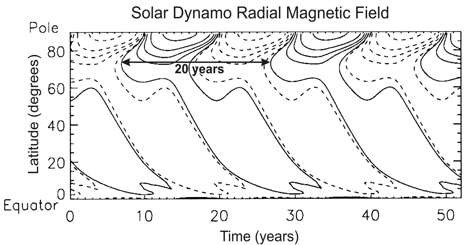
Pars pro toto, we refer here to the magneto hydro-dynamic (MHD) model of [17]. [17] generate the solar oscillation with a zonal-mean magnetic field model, which produces the solar oscillation shown in Figure 5. In this model, the poloidal (radial) magnetic field is wound up by solar differential rotation to produce a toroidal (longitudinal) field in the tachocline below the convective envelope. The buoyant toroidal field emerges at the top of the convection region to form sunspots. In that process, the Coriolis force is twisting the toroidal field to regenerate the poloidal field.
[17] artificially add in their equation for the poloidal magnetic field a nonlinear term presented here in a Taylor series expansion with variable Bf(rc,θ,t), where Bf represents the toroidal magnetic field, (r,θ) are spherical polar coordinates (rc, for the tachocline region), and Bo is taken to be constant,
 (1)
(1)
 (a) (b)
Figure 5.Shown is the radial magnetic field varying with a period of 20 years. Solid (dashed) contours correspond to positive (negative) magnetic fields, which are spaced logarithmically, with three contours covering a decade of field strength. Figure is taken from the MHD dynamo model of [17].
The nonlinear source terms of Eq.1 have the property that they are of odd (e.g., 3rd) power, a similar nonlinearity also appears in the classical dynamo model of [18]. In dynamo models, the nonlinear terms have the character of the momentum source (Figure 3) that generates the quasi-biennial oscillation (QBO). The QBO and solar dynamo have furthermore in common that the oscillation periods are determined by the dissipation rates. For the QBO, it is the eddy viscosity; and in the MHD model of [17], the magnitude of the dissipating meridional circulation mainly controls the period of the solar cycle.
3. INSECT FLIGHT
Insect flight is an outstanding example of autonomous oscillation, and the muscle physiology involved has served as a model for understanding the human heart.
In an advanced class of insects, wing frequencies as large as 1000 Hz are produced, which are determined by the inertia of the wings and far exceed the frequency capacity of the animals’ neural system [19]. This autonomous flight mechanism is produced by stretchactivation of muscle contraction [20,21], which is also important for the mammalian heart. Insect flight is very demanding energetically, and stretch-activation proves to be well suited to match the wing frequency to the aerodynamic load, making the insect “one of the most successful animals that have conquered air” [22]. In this fascinating class of insects, the flight muscles are integrated into the animal’s elastic thorax (Figure 6), changing its shape. They are therefore referred to as indirect flight muscles. The pair of dorsoventral muscles (Figure 6(a)) contract and pull the tergal plate at the back of the insect down, which causes the hinged wings to flip upwards. The longitudinal muscles (Figure 6(b)) run horizontally and compress the thorax from front to back, which causes the thorax to bow upwards and make the wings flip downwards. These antagonistic pairs of flight
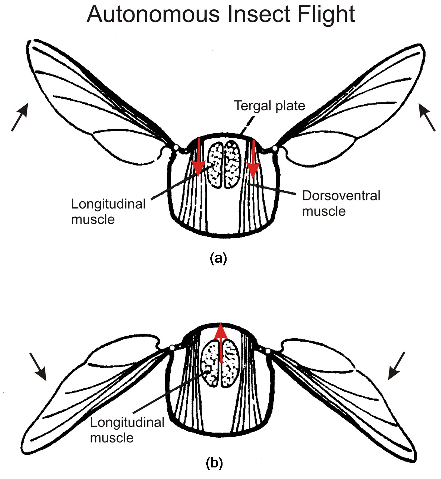
Figure 6. Insect cross-sections illustrate (a) contraction by the dorsoventral muscles that pull the tergal plate down to make the hinged wings move up, and (b) contraction of the longitudinal muscles that push the tergal plate up and the wings down. Figures taken from [23].
muscles work in tandem through stretch-activation. When the dorsoventral muscle contracts to lift the wings up (Figure 6(a)), the longitudinal muscle is stretched to activate its contraction that pulls the wings down (Figure 6(b)), and vice versa. The two antagonistic muscles alternately stretch and contract. Stretch activates the muscle contractions that force the wings up and down to produce the high frequency oscillation of autonomous insect flight. Nerve impulses command the insect flight but at a rate much slower than the wing oscillation; hence it is referred to as asynchronous flight.
4. HUMAN HEART
A tutorial review is presented of the human heart function, which provides the framework for the notion that the autonomous heart can be understood as a nonlinear oscillator.
4.1. Heart Physiology
In the cardiovascular system [24], illustrated in Figure 7, the human heart exchanges blood with the pulmonary and systemic circuits that complement each other. Oxygen-rich and CO2-poor blood, returning from the lungs in veins, is pumped in arteries by the left side of the heart to the tissue cells of the human body. The returning blood in veins, oxygen-poor and CO2-rich, is pumped in arteries by the right heart into the lungs that pick up oxygen and shed CO2.
Figure 8 illustrates the human heart anatomy. The heart functions through the interplay between the receiving chambers, the atria, and the main pumping chambers,
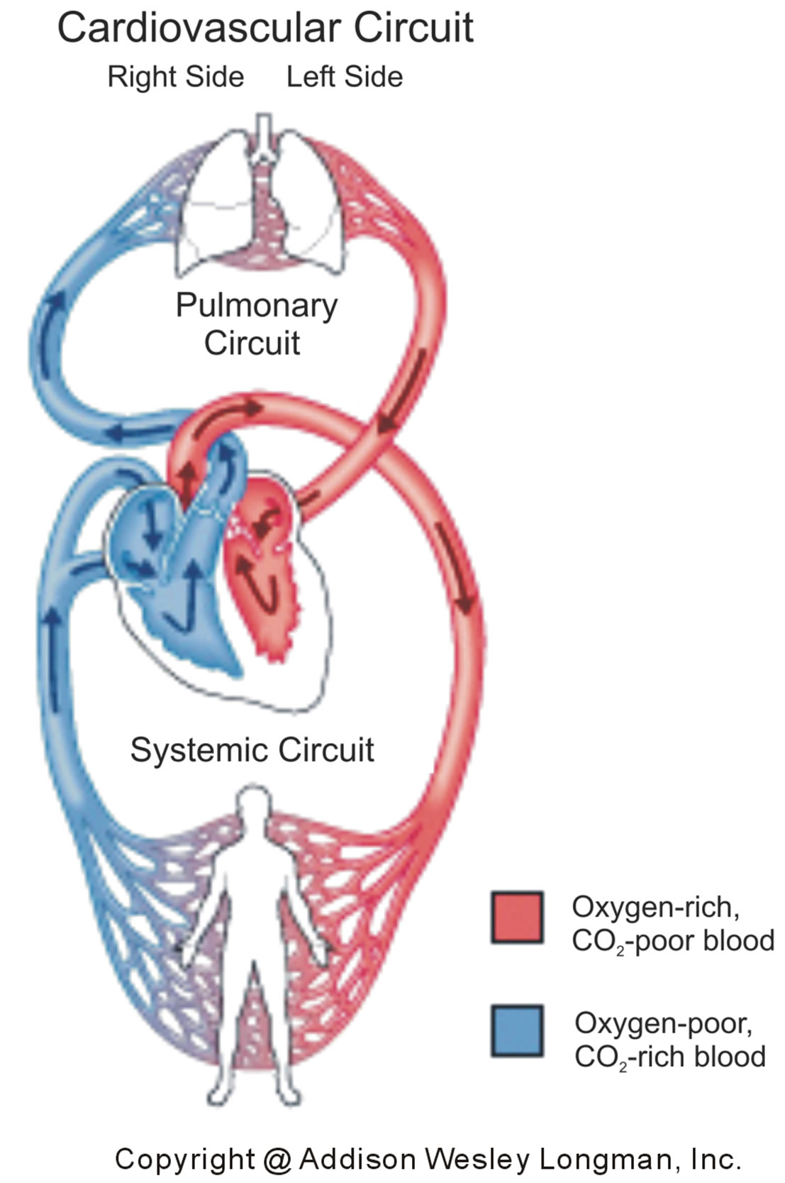
Figure 7. Pulmonary (top) and systemic (bottom) circuits of the cardiovascular system. The left side of the heart receives in veins oxygen-rich and CO2-poor blood (red) from the lungs, which is pumped in arteries to the tissue cells of the body. The right side of the heart receives in veins oxygenpoor and CO2-rich blood (blue) from the body, which is pumped in arteries to the lungs.
the ventricles, which are activated by the myocardium heart muscles. Oxygen-rich blood from the lungs returns in veins, fills the left atrium, and enters through the mitral valve into the left ventricle. And the left ventricle pumps the blood through the aortic valve and arteries to the main body tissues. On the right side of the heart, the returning oxygen-poor blood in veins fills the atrium and enters through the tricuspid valve into the right ventricle, which pumps the blood through the pulmonary valve into the arteries of the lungs. During the diastolic phase of the heartbeat, blood enters the expanding ventricles. During the systolic phase, the contracting ventricles then pump the blood with increased pressure into the lungs and the rest of the body—and Figure 9 describes the physical signatures that characterize the cardiac cycle associated with the actions inside the left side of the heart.
As illustrated in Figure 9, the closure of the aortic valve, audible in the phonogram, signals the start of the diastolic phase of the heart rhythm. Blood from the previous cardiac cycle is prevented from returning to the heart, and the muscle of the left ventricle is relaxed, occupying a minimum volume of about 50 ml (The left atrium is also relaxed at reduced volume). With the opening of the mitral valve, the main diastolic phase of the ventricle is activated. Blood returning from the lungs rapidly flows through the atrium into the left ventricle causing it to expand. At some point during this phase of

Figure 8. In the human heart, the left and right atria are filled with blood returning in veins (equipped with valves) from the lungs and main body tissues, respectively. Blood is pumped through the mitral and tricuspid valves into the corresponding ventricles. The ventricles pump the blood through the aortic and pulmonary valves into the main body tissues and lungs, respectively. The pumping actions are provided by the myocardium muscles surrounding the atria and ventricles. Figure taken from Wikipedia.
expansion, the left atrium begins to contract, and the atrium pressure increases. During the atrial systole, blood is actively pumped through the mitral valve into the ventricle, causing it to expand further. Eventually, the pressure in the ventricle becomes large enough to counter the atrium pressure, and this brings the incoming flow to a halt, causing the mitral valve to close. Under enhanced pressure, the ventricle has expanded to the peak volume of about 130 ml, almost three times the value at the beginning of the diastolic phase.
As shown in Figure 9, the systolic phase of the ventricle starts with the closing of the mitral valve, audible in the phonogram. At this point, the blood pressure abruptly increases as the ventricle contracts, evident in the decreasing volume. Following that event after a short period of time, the pressure is large enough to open the aortic valve, and the blood is ejected into the human body. At the end of the systolic phase, the ventricle then relaxes with decreasing volume, and the blood pressure goes down. Below a certain value of the ventricle pressure, the aortic pressure closes the aortic valve, and the systolic phase comes to an end.
The above-described features of the cardiac cycle apply to the left heart, which supplies the human body with oxygen-rich blood received from the lungs. The same kinds of features are also involved in the functioning of the right heart, which delivers to the lungs the oxygenpoor blood taken from the rest of the human body. The physical demands on the pumping actions of the right atrium and ventricle though are weaker than those on the left side.

Figure 9. For the left side of the heart, the time variations for the observed pressure and volume of aorta, atrium and ventricle. Also shown are the electrocardiogram and phonogram signals. Different phases of the cardiac cycle are marked by the opening and closing signals of the aortic and mitral valves and by the abrupt variations of blood pressure/volume. Figure taken from Wikipedia.
4.2. Cardiac Pacemaker
In contrast to the skeletal muscle, the cardiac muscle has its own conduction system and is not controlled by central nerves. The autonomic portion of the peripheral nervous system can control the human heart, such that sympathetic nerves initiate the cardiac response to “flight or fight”, and parasympathic nerves calm it down. Basically, the human heart functions autonomously, and its autorythmic contractions occur spontaneously. Located in the right atrium, the muscle cells of the sinoatrial (SA) node act like a cardiac pacemaker. The electric impulses generated by the SA node are associated with the contraction of the atria. After a short delay, the impulses then spread through the atrioventricular node (AV), located between the right and left atria, and then reach a large group of muscle fibers enclosing the right and left ventricles. These impulses are associated with the contraction of the ventricles. The impulse transmission through the heart’s conduction system is detected in electrocardiograms (Figure 9), where the P wave signals the atrial contraction, and the QRS wave signals the delayed contraction of the ventricle.
The cardiac pacemaker displays features that resemble the nonlinear clock mechanism illustrated in Figure 1. In the mechanical clock, the escapement mechanism produces an impulse for each swing direction to keep the pendulum oscillating at the resonance frequency. Like the nonlinear features of the clock mechanism, nonlinearity is evident in the impulse sequence of the EKG and in the abrupt variations of the ventricle blood pressure/ volume (Figure 9), discussed in the literature [25-32]. The question is what is the physiological mechanism that produces the nonlinear signatures of the autorythmic heart function.
4.3. Muscle Cell Physiology
The sarcomere is the basic building block of the muscle cell, and its physiology has recently been reviewed [33]. Illustrated in Figures 10(a) and (d), the principal protein structures of the sarcomere are the elongated thick myosin and thin actin protein filaments. First observed with high resolution electron microscopes [34,35], the two filaments in the stretched and extended sarcomere (Figure 10(a)) slide past each other to produce the shortened configuration (Figure 10(d)) of the muscle contraction. In this sliding action, the titin protein acts like a sponge.
At the molecular level, the mechanism of muscle contraction is illustrated in Figures 10(b) and (c). During contraction, the myosin heads attach to the actin proteins and pull them towards the middle of the sarcomere. Actin filaments slide past myosin filaments, and the sarcomere shortens. The process is regulated by two proteins, tro-

Figure 10. The sarcomere is made up of elongated actin and myosin protein filaments, shown for the stretched/relaxed (a) and contracted (d) muscle. In the stretched sarcomere, the tropomyosin protein covers the actin and blocks the myosin interaction (b). Ca++ and troponin protein combine to dislodge the tropomyosin. This opens the actin globules to the myosin interaction, which is produced by cross-bridges that attach to the actin filament and drag it to the center of the sarcomere, hence shortening it (c). Adenosin triphosphate (ATP) provides the energy for the sarcomere contraction. Figures taken from Wikipedia, and www.ucl.ac.uk.
pomyosin and troponin. Tropomyosins are coiled proteins that run along the actin filament, where they can cover the binding sites for myosin and thus block the muscle contraction (Figure 10(b)). Calcium from the sarcoplasma is required for the muscle contraction. The Ca++ ions bind with the troponin complex, which reconfigures the tropomyosin such that the globular actin proteins become exposed to the myosin heads (Figure 10(c)). Myosin heads then deliver the mechanical force for muscle contraction. That force is produced by so called cross-bridges [36,37], which are hinged elements of the myosin heads that bend and attach to actin, and then drag the actin filament to produce muscle contraction. The energy required for this force is provided by adenosin triphosphate (ATP) molecules that attach to myosin heads. ATP is unstable in water. When ATP is hydrolized, the bond connecting the phosphate is broken to produce adenosin diphosphate (ADP), and energy is released. The chemical energy thus liberated powers the bending myosin heads that push the actin filaments (Figure 10(c)) to produce the sarcomere muscle contraction.
4.4. Starling’s Law of the Heart and Stretch-Activation of Muscle Contraction
We believe that the nonlinearity of the heart function is manifest in the stretch-activation of cardiac muscle contraction, consistent with Starling’s Law of the Heart.
In a series of laboratory experiments with dogs led by Starling [38], the team of scientists observed that the increasing blood in veins filling the cardiac ventricle led to increased stroke volume caused by muscle contraction. This property of the cardiovascular system is found in animals and humans, and it is independent of neural influences on the heart. In mechanical terms, Starling’s law implies that the initial stretching of the cardiac muscle affects contraction. The more the muscle is stretched the greater the force of contraction. As a result, the heart naturally adapts to the physiological condition and demands of the body, Starling’s Wisdom of the Body. Quoting Wikipedia, Starling’s Law of the Heart states that the stroke volume of the heart increases in response to an increase in the volume of the blood filling the heart (the end diastolic volume). The increased volume of the blood stretches the ventricular wall, causing the cardiac muscle to contract more forcefully.
Stretch-activation of muscle contraction is a pronounced, and outstanding, feature of insect flight muscles [20,21], and significant progress has been made explaining the mechanism at the molecular level, reviewed by [22] and briefly illustrated in Section 4.3. Applying electron microscopy, [39] studied the force production of myosin cross-bridges (Figure 10(c)), separating the effects of Ca++ abundance and stretching of the sarcomere. For this experiment, the giant water bug Lethocerus was used, where isolated muscle fibers can oscillate for several hours. The experiment clearly demonstrated that stretchactivation and Ca++ ions are complementary pathways for cross-bridge attachment and force production. The data suggested that stretch-induced distortion of attached cross-bridges relieves the tropomyosin blocking (Figure 10(b)) of binding sites on actin, so that the maximum force of contraction can be generated at low calcium concentrations. Following up on this study, [40] discovered new cross-bridges between myosin and actin filaments, involving troponin, they named troponin bridges. They exposed the oscillating muscle to intense X-rays and recorded during muscle contraction the diffraction patterns associated with the positions of myosin heads, actin filaments, troponin, and tropomyosin. Based on these data, they proposed a comprehensive, self-consistent structural model for stretch-activation. When the muscle fibers are stretched, provided there is some Ca++ present, the troponin bridges assist in pulling tropomyosin away to expose the myosin binding sites on actin, thus activating contraction (Figure 10(c)). While the thin actin filaments are opened due to stretch, the thick myosin filaments are twisting in response to stretch. The result is that more myosin heads are brought to actin target zones during muscle stretch so that more cross-bridges are formed for larger force production.
In the skeletal muscle, nerve impulses stimulate the release of Ca++, which prompts the muscle contraction. Calcium is also important for the cardiac muscle but does not control its operation. Discussed by [41], the rhythmic nature of the cardiac muscle contraction calls for a functional analogy with stretch-activation of the insect flight muscle. Moreover, stretch-activation is called for by the steep length tension relationship of the cardiac muscle, which is necessary to explain Starling’s Law of the Heart [42,43]. In cardiac muscles, the importance of stretchactivation has been demonstrated [44-46]. [47] investigated the stretch-activation of cardiac muscle contraction and its dependence on the Ca++ concentration. Calcium levels were varied, and the force response to stretch was evaluated. The data showed that stretch-activation is most pronounced at low levels of calcium activation when the thin actin filament offers many sites for the formation of additional cross-bidges that can produce muscle contraction. They concluded that stretch-activation produces strong-binding cross-bridges, which in turn open up target zones for new cross-bridges on the actin filament, and thus increase the force response during muscle contraction. Another force producing pathway was pointed out by [48]. They proposed that the Ca2+ dependent sensitivity of muscle contraction can be modulated by the stretch or length dependent variations in the lateral spacing between actin and myosin filaments, which affects the formation of myosin cross-bridges. At the molecular level, [49] employed X-ray diffraction to determine the cross-bridge proximity of the myosin heads in relation to the thin actin filament. It showed convincing evidence for a reduction of spacing between the thick and thin filaments, which increased the number of crossbridges involved in the force production during the early phase of the ventricular contraction. As shown for the autonomous operation of the insect flight muscles, there is now abundant observational evidence that stretch-activation is of central importance for the cardiac muscle contraction, consistent with Starling’s Law of the Heart [38].
4.5. Nonlinear Heart Function
Given that stretch-activation explains the function of the cardiac muscle, consistent with Starling’s Law of the Heart, what justifies our picture that the heart is a nonlinear oscillator?
Referring to the introduction (Section 1), simple examples of nonlinearity are evident in the feedback of snow, which reflects the solar radiation to accelerate cooling, and in melting glaciers due to CO2-induced global warming, which further accelerates warming. Nonlinearity is also apparent in the oscillation of fluid streaming out of a bottleneck, being chocked by pressure feedback. From the numerical results discussed in Sections 2.1 and 2.2, we learn that the nonlinear interactions between gravity waves, x, and winds, y, produce the steep nonlinear momentum source, xy, shown in Figures 3 and 4(b), respectively.
In the case of the human heart, the diastolic built up of the ventricle blood pressure and resulting stretching of the muscle sarcomere (Figure 10(a)) could be viewed as variable, x. The stretch induced formation of myosin cross-bridges (Figure 10(c)), discussed in Section 4.3, could be the other variable y, which produces the muscle contraction and built-up of systolic blood pressure. Since stretch induces muscle contraction, more stretch produces more muscle contraction, we believe that the nonlinear nature of the heart function seems well established. Nonlinear signatures of this interaction are seen in abrupt variations of the ventricular blood pressure and volume (Figure 9), and in the electrocardiogram that signals different phases of the cardiac cycle (Figure 9), as discussed in the literature [25-32]. In our picture of the autonomous human heart, the rhythmic oscillation is produced by the nonlinearity built into the stretch activated contraction of the cardiac muscles, consistent with Starling’s Law of the Heart. This physiological mechanism could prompt the pacemaker signals, seen in electrocardiograms, which are transmitted through the cardiac conduction system to coordinate and synchronize the muscle functions. Like the nonlinear clock that needs to be activated initially to start oscillating, the human heart needs to be pumped up to start functioning again.
The above stretch-activation of muscle contraction applies to the ventricles, the main pumping chambers of the heart. The atria that pump the blood into the ventricles during the atrial systol, as seen in the blood pressure diagram (Figure 9), are the complementary antagonists to the ventricles. As the muscles in the atria contract, the muscles in the ventricles stretch, analogous to the earlier discussed stretching and contraction of the antagonistic autonomous insect muscles (Section 3, Figure 6). The atria could be seen as being stretched by the blood returning in the venous system of the pulmonary and systemic circuits of the human body (Figures 7 and 8). And stretching of the atria could induce atrial contraction to produce the other nonlinear component of the oscillating heart, thus complementing the nonlinear stretch activation of the ventricles.
For the heart to oscillate, an antagonistic and complementary counter-part is required to oppose the pumping action during the systolic phase. The blood in veins with valves (Figure 8), returning from the lungs and the rest of the body, must be pumped into the atria during the diastolic phase (Figure 9). This pumping action is provided by: 1) the contraction of skeleton muscles and pulmonary pump that squeeze the elastic veins; 2) the contraction of smooth muscles surrounding the enervated veins, which is prompted by the sympathetic nervous system that responds to the stress and demands of the body; and 3) perhaps, the stretch induced contraction of the veins’ smooth muscles in response to the built-up of blood pressure.
5. CONCLUDING REMARKS
The fluid dynamical oscillators discussed have been simulated with nonlinear numerical models. In the quasibiennial oscillation (QBO) and bimonthly oscillation (BMO), the gravity wave interactions with the atmospheric circulation produce momentum sources that are strongly nonlinear as shown respectively in Figure 3 and Figure 4(b). For the solar dynamo model, a nonlinear source term (Eq.1) is employed to generate the 22-year oscillation. These nonlinear autonomous oscillators were not controlled, and constrained, by external time dependent forcing. The periods of their oscillations are solely determined by the internal dynamical properties of the fluids.
Numerical results for the QBO (Figure 2) show that the amplitude and period of the oscillation are reduced by about a factor of two when the dissipating viscosity is increased by that factor. The period of the BMO (Figure 4) is generated by the thermodynamic feedback of the meridional winds. In the solar dynamo model [17], the oscillation period of the magnetic field (Figure 5) varies inversely with the magnitude of the dissipating meridional circulation. The physical properties of these fluid dynamical oscillators resemble those of the nonlinear human heart, which is affected by the constraints and demands of the body. With arterio sclerosis due to narrowing of the arteries for example, the heart experiences more resistance in delivering the blood. As a result, the heart rate increases, and the volume of blood delivered in each stroke decreases—analogous to the changing QBO in response to the increased rate of dissipation.
The nonlinear fluid dynamical oscillators discussed were chosen to function autonomously without external time dependent source. The mechanical clock was not shaken, and the QBO was not forced externally by time dependent solar heating. In reality, numerical experiments show that, under the name of a pacemaker, the seasonal variations amplify the QBO and modulate its periodicity [50,51]. The human heart does not function solely through stretch-activation. The heart functions in concert with the vascular system, where sympathetic nerves activate the smooth muscles around enervated veins that pump the blood to the heart, in response to stress or exercise for example. This autonomous, and harmonic, function of the human heart can be interrupted by sympathetic nerves that can initiate the cardiac response to “flight or fight”, and by parasympathetic nerves that calm down the heart.
The basic physical processes involved in describing the present fluid dynamical oscillators are well understood. To obtain global-scale numerical computer solutions, a parameterization algorithm was employed to simulate the gravity wave interactions that generate the QBO and BMO, and a nonlinear source term was introduced to generate the solar dynamo oscillation.
Compared to the nonlinear oscillators in space physics, the multifaceted operation of the human heart and cardio-vascular system is far more complicated. To deal with that complexity, one could envision parameterizetion schemes that describe the observed properties of stretch activated muscle contraction at the molecular level. Nonlinearity would come into play by allowing stretching to influence contraction in the atrial and ventricle heart chambers (Figure 8). To produce the oscillation would require that the heart is made to interact with the vascular system (Figure 7). This antagonistic and complementary process to the heart function would require a parameterization that describes the volume of returning venous blood in relation to the stress and demands of the human body, satisfying Starling’s Law of the Heart and Wisdom of the Body. Dissipation would have to be built into the model, allowing for example for the resistance the blood experiences in the arteries, analogous to the viscous dissipation of the QBO and friction in the mechanical clock.
The complex cardio-vascular system could perhaps be compared with the weather systems near the ground and in space, where a multitude of nonlinear interactions produce a complex phenomenology. Physics based numerical mathematical models, aided by parameterizations, have greatly advanced our understanding of the environment to produce powerful predictive capabilities. Considering the enormous advances made in describing and understanding the heart physiology, we believe that the next decade will probably see mathematical models that can simulate the operation of the human heart.
6. ACKNOWLEDGEMENTS
The authors are indebted to an anonymous reviewer and to Dr. Kenneth Schatten for valuable comments that contributed significantly to improve the presentation of the paper. This work was in part supported by the NASA TIMED Contract to the Johns Hopkins Univsersity, Applied Physics Laboratory. The authors greatly appreciate the help Patricia Bowden provided in editing the manuscript.
REFERENCES
- Mayr, H.G. and Schatten, K.H. (2012) Nonlinear oscillators in space physics. Journal of Atmospheric and SolarTerrestrial Physics, 74, 44-55. doi:10.1016/j.jastp.2011.09.008.
- Baldwin, M.P., Gray, L.J., Dunkerton, T.J., et al. (2001) The quasi-biennial oscillation. Review of Geophysics, 39, 179-229. doi:10.1029/1999RG000073.
- Lindzen, R.S. and Holton, J.R. (1968) A theory of the quasi-biennial oscillation. Journal of Atmospheric Science, 25, 1095-1107. doi:10.1175/1520-0469(1968)025<1095:ATOTQB>2.0.CO;2
- Mengel, J.G., Mayr, H.G., Chan, K.L., Hines, C.O., Reddy, C.A., Arnold, N.F. and Porter, H.S. (1995) Equatorial oscillations in the middle atmosphere generated by small scale gravity waves. Geophysics Research Letters, 22, 3027-3030. doi10.1029/95GL03059
- Dunkerton, T.J. (1997) The role of the gravity waves in the quasi-biennial oscillation. Journal of Geophysical Research, 102, 26053-26076. doi:10.1029/96JD02999.
- Holton, J.R. and Lindzen, R.S. (1972) An updated theory for the quasi-biennial cycle of the tropical stratosphere. Journal of Atmospheric Science, 29, 1076-1080. doi:10.1175/1520-0469(1972)029<1076:AUTFTQ>2.0.CO;2
- Mayr, H.G., Mengel, J.G. and Chan, K.L. (1998) Equatorial oscillations maintained by gravity waves as described with the Doppler Spread Parameterization: I. Numerical experiments. Journal of Atmospheric and Solar-Terrestrial Physics, 60, 181-199. doi:10.1016/S1364-6826(97)00122-3.
- Mayr, H.G., Mengel, J.G., Hines, C.O, Chan, C.L., Arnold, N.F., Reddy, C.A. and Porter, H.S. (1997) The gravity wave Doppler spread theory applied in a numerical spectral model of the middle atmosphere 1. Model and global scale variations. Journal of Geophysical Research, 102, 26077-26091. doi:10.1029/96JD03213.
- Hines, C.O. (1997) Doppler-spread parameterization of gravity-wave momentum deposition in the middle atmosphere. Part 1: Basic formulation. Journal of Atmospheric and Solar-Terrestrial Physics, 59, 371-386.
- Hines, C.O. (1997) Doppler-spread parameterization of gravity-wave momentum deposition in the middle atmosphere. Part 2: Broad and quasi monochromatic spectra, and implementation. Journal of Atmospheric and SolarTerrestrial Physics, 59, 387-400.
- Mayr, H.G., Mengel, J.G., Reddy, C.A., Chan, K.L. and Porter, H.S. (1999) The role of gravity waves in maintaining the QBO and SAO at equatorial latitudes. Advance in Space Research, 24, 1531-1540.
- Eckermann, S.D. and Vincent, R.A. (1994) First observations of intra-seasonal oscillations in the equatorial mesosphere and lower thermosphere. Geophysics Research Letters, 21, 265-268.
- Lieberman, R.S. (1998) Intraseasonal variability of highresolution Doppler imager winds in the equatorial mesosphere and lower thermosphere. Journal of Geophysical Research, 103, 11221-11228. doi:10.1029/98JD00532.
- Huang, F.T. and Reber, C.A. (2003) Seasonal behavior of the semidiurnal and diurnal tides, and mean flows at 95 km, based on measurements from the High Resolution Doppler Imager (HRDI) on the Upper Atmosphere Research Satellite (UARS). Journal of Geophysical Research, 108, 4360-4376. doi:10.1029/2002JD003189.
- Mayr, H.G, Mengel, J.G., Drob, D.P., Porter, H.S. and Chan, K.L. (2003) Intraseasonal oscillations in the middle atmosphere forced by gravity waves. Journal of Atmospheric and Solar-Terrestrial Physics, 65, 1187-1203. doi:10.1016/j.jastp.2003.07.008.
- Schatten, K. (2005) Fair space weather for solar cycle 24. Geophysics Research Letters, 32, L21106-L21110. doi:10.1029/2005GL024363.
- Dikpati, M. and Charbonneau, P. (1999) A BabcockLeighton flux transport dynamo with solar-like differenttial rotation. The Astrophysical Journal, 518, 508. doi:10.1086/307269.
- Leighton, R.B. (1969) A Magneto-Kinematic model of the solar cycle. The Astrophysical Journal, 156, 1. doi:10.1086/149943
- Sotavolta, O. (1947) The flight-tone (wing stroke frequency) of insects. Suomen Hyönteistieteellinen Seura, 4, 1-117.
- Pringle, J.W. (1949) The excitation and contraction of the flight muscle of insects. Journal of Physiology, 108, 226- 232.
- Pringle, J.W. (1978) The Cronian Lecture, 1977: Stretch activation of muscle: Function and mechanism. Proceedings of the Royal Society B: Biological Science, 201, 107- 130.
- Merzendorfer, H. (2011) Mechanism for stretch activation proposed. Journal of Experimental Biology, 214, 4-5, doi:10.1242/jeb.049759.
- Snodgrass, R.E. (1935) Principles of insect morphology. McGraw-Hill Publishing Co., New York.
- Alcamo, I.E. and Krumhardt, B. (2004) Barron’s anatomy and physiology. Barron’s Educational Series.
- Chillemi, S., Barbi, M., Di Garbo, A., et al. (1997) Detection of nonlinearity in the healthy heart rhythm. Method of Information in Medicine, 36, 278-281.
- Chen, Z., Brown, E.N. and Barbgieri, R. (2008) Characterizing nonlinear heartbeat dynamics within a point process framework. IEEE Transactions on Biomedical Engineering, 57, 2781-2784. doi:10.1109/TBME.2010.2041002.
- Korhonen, I.K.J. and Turjanmaa, V.M.H. (1995) Secondorder non-linearity of heart rate and blood pressure shortterm variability. Computers in Cardiology, Lyon, 10-13 September 1995, 293-296.
- Guzzetti, S., Signorini, M.G., Cogliati, C., et al. (1996) Non-linear dynamics and chaotic indices in heart rate variability of normal subjects and heart transplanted patients. Cardiovascular Research, 31, 441-446.
- Perc, M. (2005) Nonlinear time series analysis of the human electrocardiogram. European Journal of Physics, 26, 757-768. doi:10.1088/0143-0807/26/5/008.
- Kuusela, T.E., Jarttii, T.T., Tahvanainen, K.U.O. and Kaila, T.J. (2002) Nonlinear methods of biosignal analysis in assessing terbutaline-induced heart rate and blood pressure changes. American Journal of Physiology: Heart and Circulatory Physiology, 282, H773-H781.
- Jo, J.A., Blasi, A., Valladares, E.M., et al. (2007) A nonlinear model of cardiac autonomic control in obstructive sleep apnea syndrome. Annals of Biomedical Engineering, 35, 1425-1443,
- Riedl, M., Suhrbier, A., Malberg, H., et al. (2008) Modeling the cardiovascular system using a nonlinear additive autoregressive model with exogenous input. Physical Review E, 78, 100919. doi:10.1103/PhysRevE.78.011919.
- Krans, J.L. (2010) The sliding filament theory of muscle contraction. Nature Education, 3, 66.
- Huxley, H.E. and Niedergerke, R. (1954) Structural changes in muscle during contraction: Interference microscopy of living muscle fibres. Nature, 173, 971-973.
- Huxley, H.E. and Hanson, J. (1954) Changes in the crossstriations of muscle during contraction and stretch and their structural interpretation. Nature, 173, 973-976.
- Hynes, T.R., et al. (1987) Movements of myosin fragments in vitro: Domains involved in force production. Cell, 48, 953-963. doi:10.1016/0092-8674(87)90704-5.
- Spudich, J.A. (2001) The myosin swinging cross-bridge model. Nature Reviews Molecular Cell Biology, 2, 387- 392. doi: 10.1038/35073086
- Starling, E.H., (1923) The Harveian oration on the “Wisdom of the Body”. Lancet, 202, 865-870.
- Linari, M., Reedy, M.K., Reedy, M.C., Lombardi, V. and Piazzesi, G. (2004) Ca-activation and stretch-activation in insect flight muscle. Biophysical Journal, 87, 1101-1111. doi:10.1529/biophysj.103.037374.
- Perz-Edwards, R.J., Irving, T.C., Baumann, B.A., et al. (2010) X-ray diffraction evidence for myosin-troponin connection and tropomyosin movement during stretch activation of insect flight muscle. Proceedings of the National Academy of Sciences of USA, 108, 120-125. doi:10.1073/pnas.1014599107.
- Campbell, K.B. and Chandra, M. (2006) Functions of stretch activation in heart muscle. The Journal of General Physiology, 127, 89-94. doi:10.1085/jgp.200509483.
- Solaro, R.J. (2007) Mechanisms of the frank-starling law of the heart: The beat goes on. Biophysical Journal, 93, 4095-4096. doi:10.1529/biophysj.107.117200.
- Allen, D.G. and Kentish, J.C. (1985) The cellular basis of the length-tension relation in cardiac muscle. Journal of Molecular and Cellular Cardiology, 17, 821-840.
- Steiger, G.J. (1971) Stretch activation and myogenic oscillation of isolated contractile structures of heart muscle. Pflugers Archiv, 330, 347-361.
- Steiger, G.J. (1977) Stretch-activation and tension transients in cardiac, skeletal and insect flight muscle. In: Tregear, R.T. Ed., Insect flight muscle, Elsevier, Amsterdam, 221-268.
- Vemuri, R., Lankford, E.B., Poetter, K., et al. (1999) The stretch-activation response may be critical to the proper functioning of the mammalian heart. Proceedings of the National Academy of Sciences of USA, 96, 1048-1053.
- Stelzer, J.E., Larsson, L., Fitzsimons, D.P. and Moss, R.L. (2006) Activation dependence of stretch-activation in mouse skinned myocardium: Implications for ventricular function. The Journal of General Physiology, 127, 95-107. doi:101085/jgp.200509432.
- Fuchs, F. and Smith, S.H. (2001) Calcium, cross-bridges, and the Frank-Starling relationship. News in Physiological Science, 16, 5-10.
- Pearson, J.T., Shirai, M., Tsuchimochi, H., et al. (2007) Effects of sustained length-dependent activation on in situ cross-bridge dynamics in rat hearts. Biophysical Journal, 93, 4319-4329. doi:10.1529/biophysj.107.111740.
- Mayr, H.G, Mengel, J.G., Reddy, C.A., Chan, K.L. and Porter, H.S. (2000) Properties of QBO and SAO generated by gravity waves. Journal of Atmospheric and SolarTerrestrial Physics, 62, 1135-1154. doi:101016/S1364-6826(00)00103-6.
- Mayr, H.G., Mengel, J.G., Chan, K.L. and Huang, F.T. (2010) Middle atmosphere dynamics with gravity wave interactions in the numerical spectral model: Zonal-mean variations. Journal of Atmospheric and Solar-Terrestrial Physics, 72, 807-826. doi:10.1016/j.jastp.2010.03.018