Engineering
Vol.09 No.03(2017), Article ID:75189,37 pages
10.4236/eng.2017.93016
Impact of Reservoir Properties on the Production of the Mannville Coal Measures, South Central Alberta from a Numerical Modelling Parametric Analysis
Amanda M. M. Bustin, Robert Marc Bustin
Department of Earth, Ocean and Atmospheric Sciences, The University of British Columbia, Vancouver, Canada

Copyright © 2017 by authors and Scientific Research Publishing Inc.
This work is licensed under the Creative Commons Attribution International License (CC BY 4.0).
http://creativecommons.org/licenses/by/4.0/


Received: January 28, 2017; Accepted: March 28, 2017; Published: March 31, 2017
ABSTRACT
Numerical simulations are used to investigate the impact of intrinsic and extrinsic reservoir properties on the production from coal and organic rich lithologies in the Lower Cretaceous Mannville coal measures of the Western Canadian Sedimentary Basin. The coal measures are complex reservoirs in which production is from horizontal wells drilled and completed in the thickest coal seam in the succession (1 m versus 3 m), which has production and pressure support from thinner coals in the adjacent stratigraphy and from organic-rich shales interbedded and over and underlying the coal seams. Numerical models provide insight as to the relative importance of the myriad of parameters that may impact production that are not self-evident or intuitive in complex coal measures.
Keywords:
Coal Bed Methane, Gas Shales, Parametric Analysis, Reservoir Modelling, Unconventional Reservoirs

1. Introduction
Coal gas production of stratigraphically and structurally complex coal measures is dependent on a myriad of interrelated variables. Hence, isolating the contribution of intrinsic and extrinsic variables to productivity is challenging at best and commonly impossible. In coal measures, such as those of the Lower Cretaceous, Mannville Group, in the Western Canadian Sedimentary Basin, where multiple coal seams and organic rich shales occur, the problem is further compounded. In an attempt to better understand the relative importance of controls on well productivity, we have investigated the variation in producability of coals and associated organic rich gas shales through a parametric analysis using a numerical modelling program, which simulates gas and water production. The numerical models are grounded in field and laboratory analyses of coals throughout the producing Mannville fairway in Alberta [1] .
In previous studies, the fabric of the reservoir, which includes the fracture network as well as the microfabric of the matrix, has been shown to control producability of both coals and shales (e.g. [2] [3] ). The fracture network controls both the fracture permeability and the path length for gas transport through the matrix, while the microfabric of the matrix controls the rate of gas transport through the matrix. The production potential of the coal and shale layers is most sensitive to fracture permeability, which depends on the fracture spacing, fracture aperture, and relative fluid saturation. In comparatively weak coals, significant dynamic changes in the fracture permeability can also occur with gas production as a result of matrix shrinkage (i.e., fracture dilation), due to gas desorption, as well as matrix swelling (i.e., fracture compaction) with increasing stress, due to reservoir pressure depletion ( [4] [5] ). Understanding the dynamic changes in coal fracture permeability requires knowledge of the mechanical properties and the volumetric strain associated with gas desorption.
In the producing Mannville coal measures in south-central Alberta (Figure 1), production is mainly from horizontal wells drilled and completed in the thickest coal seam in the succession (Figure 1(c)). Significant gas, generally not considered in the total gas-in-place calculations, is present within adjacent coal seams and high organic content, fine-grained strata (referred to here as gas shales) that are interbedded with or under and overlie the coals (Figure 1(a)). References [1] and [6] showed that 63% of the total calculated gas-in-place in the Upper Mannville coals is contained within the minor coal seams, including the shales increases the total gas-in-place 1.7 times that of the coals (Figure 1(d)). Reference [7] presented numerical simulations, showing that the minor coal seams increase the recovered gas by 1.4 times (×) and the recovered water by 3.0×, while the shale beds result in 1.7× more produced gas and 2.5× more produced water after 25 years of production than when only the main coal seam is considered.
In this study, the importance of the gas content and fabric parameters of both the coal and shale layers on production are quantified, compared, and ranked through a parametric analysis. Experimental and field data from the Mannville coal measures and adjacent shales in the Corbett region in south-central Alberta (Figure 1(b)) are used as model inputs for a general equation-of-state reservoir simulator (CMG-GEM). The parametric analysis was performed by systematically varying all model parameters, between their maximum and minimum values determined from the data compilation. A constant coal fracture permeability was input for the first stage of the parametric analysis, following which a stress-dependent coal fracture permeability model was used and the impact of the coal fracture compaction/dilation parameters on the productivity was also investigated. The impact of the parameters varies with production, often in
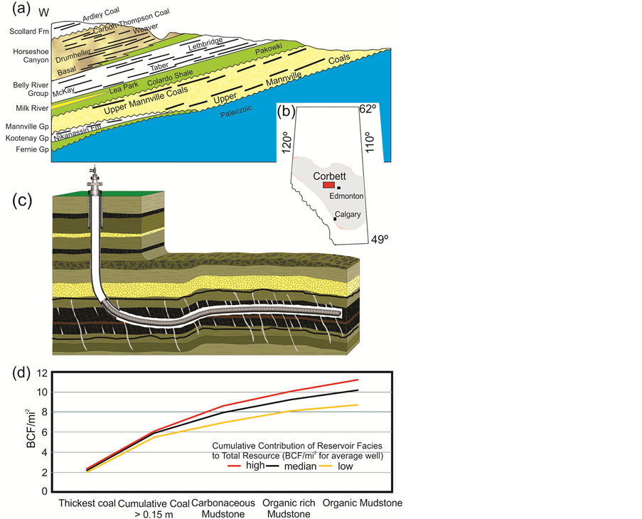
Figure 1. (a) Schematic cross-section across the Western Canadian sedimentary basin (modified from [8] ). (b) Mannville coal distribution in Alberta shown as the grey region and the location of the Corbett fairway, shown as the red rectangle (modified from [9] ). (c) Schematic diagram of a single horizontal well, 1000 - 1600 m long, drilled and completed in the main (i.e., thickest) coal seam in the sequence (modified from [10] ). (d) Cumulative resource by BCF/section for the P10, P50, and P90 gas contents showing the contribution of the main coal seam, all coal seams >0.15 m, and the shales (variably organic mudstones) for the Mannville coal measures (modified from [6] ).
complicated ways and while most of the results were anticipated, some are not intuitive. A better understanding of the impact of the coal and shale parameters on well productivity provides insights for reserve analysis and for optimising well spacing units, lateral lengths, and orientations.
2. Model Parameters
The model parameters for this study were compiled from existing industry and academic databases as well as from new laboratory tests on coal and shale samples collected from three Mannville wells: 12-31-62-05W5, 15-27-62-06W5, and 16-10-62-06W5. The production was simulated from a single 1000 m long horizontal well centered within a 6400× 6400 m model, discretized into 100 m grid blocks. The horizontal well is oriented within the model perpendicular to the direction of the maximum coal fracture permeability, which based on field data is known to be anisotropic, due to the anisotropy of the far field stress (Figure 2(c)). The depth and thickness of the horizontally stacked coal seams in the models, determined from interpretations of logs from well 16-10-62-06W5, are shown in Table 1. During the parametric analysis, the production for the model with the coal geometry from well 16-10-62-06W5 was compared to the production for models with coal geometries from the 12-31-62-05W5 and 15-27-62- 06W5 wells, which are also shown in Table 1. Layers (beds) of gas shales are interbedded with the coal layers, with thickness varying from 1.1 m to 20 m. In the model design, shale layers 20 m thick were also added for 200 m above and 400 m below the reservoir, resulting in a model extending from 745 to 1415 m in depth. A cross-section of the model showing the geometry of the coal versus shale layers is shown in Figure 2. The original-gas-in-place (OGIP) within the wet (Sw > 0) Mannville Group is in the adsorbed state while the cleats and fractures are 100% water-saturated.
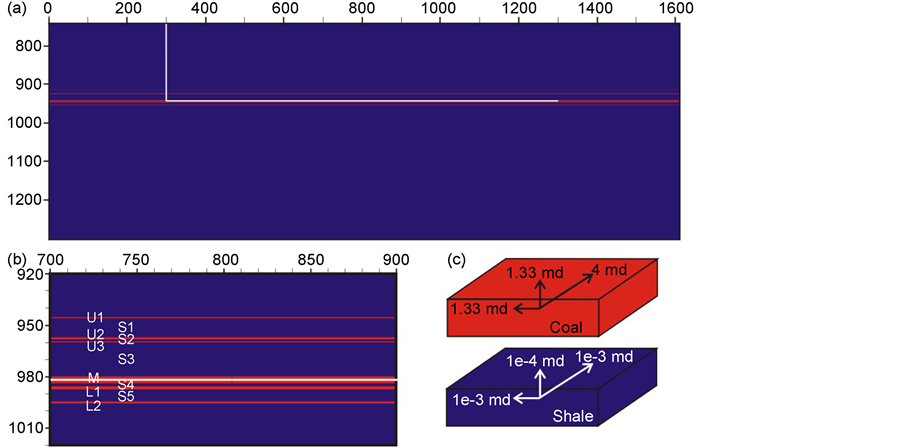
Figure 2. Cross-section of the model through a plane containing the wellbore showing the geometry of the coal seams (red) versus shale layers (blue); (a) Cross-sectional view of the full model and (b) close-up of the reservoir. The labels for the coal seams and interbedded shale layers are shown on; (b) The location of the horizontal well is shown by thin white lines; (c) Three-dimensional schematic illustrating the coal (top) and shale (bottom) fracture permeability anisotropy.

Table 1. Depth to top of coal seams and seam thickness in the 3 Mannville wells.
Estimates of the parameter values for each lithologic unit are not available and, since accurate production forecasting and history matching are not the goals of the modelling, the model parameters were averaged such that each coal seam, while having unique geometry, is assigned equal parameter values. All the shale layers were also assigned equal parameter values, which were chosen from the statistics of measured values from all shales. When appropriate, probability distributions were calculated for the parameter values by first fitting a normal distribution to each dataset and then performing a Monte Carlo simulation. The average values were thus chosen as the 50% probability (P50). Insufficient data exists for several of the parameters, in these cases simple arithmetic averages were calculated (parameters with n < 15 in Table 2). Lacking methods for accurate field measurements, the effective fracture spacings were estimated from historical knowledge of unconventional reservoirs and the fracture porosities were estimated from the match-stick model ( [11] [12] ).
During the parametric analysis, the models with end-member parameter values were systematically compared. The end-member values were chosen as the
Table 2. The input parameters used during the modelling.
Note the matrix porosity values listed above were assumed during the modelling, due to the bound matrix water (matrix Sw assumed to be zero in the model), and are not the measured values. Dynamic changes in fracture permeability were only considered for the coals, thus no rock mechanics or volumetric strain parameters were input for the shales.
P10 and P90 values when a probability distribution was calculated for the parameter; otherwise, they were chosen as the maximum and minimum values. The average, minimum, and maximum parameter values used as model inputs as well as the number of data points available for each parameter are tabulated in Table 2.
3. Results
The reservoir modelling in this study was carried out using the commercial CMG’s GEM advanced general equation-of-state compositional simulator. The sensitivity of the producability of the Mannville reservoir from a 1000 m long horizontal well to the coal and shale parameters was investigated through a parametric analysis. The base model for the parametric analysis is the model with average parameter values and during the analysis, each coal and shale parameter was systematically varied between end-member values, while all the other parameters are held at their average values and the resulting production over a 10 year history were compared. The impact of the parameter was quantified as the ratios between the gas and water cumulative production predicted for the models with end-member parameter values. The ratio of gas recovered from the shale layers versus the coal seams increases for all models over the production history. The impact on the ratios of the gas recovered from shale versus coal layers at the end of the 10 year production history were also quantitatively compared for the end member models. The fracture permeability of the coals was initially assumed to be independent of changes in porosity during production to investigate the effect of the coal and shale parameters. The parameters in the first part of the analysis include the Langmuir parameters, matrix permeability, fracture permeability, fracture spacing, and fracture porosity for both the coals and the shales. The modelling results predict that the shale fracture porosity, shale fracture spacing, and coal matrix permeability have low impacts on cumulative gas and water production as well as the ratio of recovered shale to coal gas (all impacts ≤ 1.1x). While the results for these parameters are included in summary plots, they are not further discussed in this paper. The results from the average model were also compared to those simulated for models with the coal geometries from the 12-31-62-05W5 and 15-27-62-06W5 wells, in order to understand the influence of the depth and thickness of the coal seams on the producability.
The second part of the parametric analysis investigates the impact of dynamic changes in coal fracture permeability on production. The net importance of matrix swelling with increasing effective stress versus matrix shrinkage with gas desorption on the coal fracture permeability was determined as well as the sensitivity of production to the Young’s modulus, Poisson’s ratio, volumetric strain, and half-strain pressure. In comparison to the other coal fracture compaction/dilation parameters, the half-strain pressure has a much lower impact on the gas and water production and while the results are included in summary plots, they are not further discussed.
3.1. Comparison of Wells
The variation in production between the average model (16 - 10) and models created from the coal seam depths and thicknesses from the 12-31-61-06W5 well (12 - 31) and 15-27-62-06W5 well (15 - 27) was investigated. The parameter values are the same for the 12 - 31 and 15 - 27 models as the average model except for the depth and thickness of the strata, which were determined from the well logs. The 12 - 31 and 15 - 27 wells both have thinner main coal seams than the 16 - 10 well and one less upper coal seam, resulting in lower net coal thickness (8.8 m and 6.3 m versus 9.1 m; Table 1). The coal seams in the 12 - 31 well are shallower and extend over a larger depth range than the coal seams in the 16 - 10 well, which are shallower and extend over a larger depth range than the 15 - 27 well. While the coal seams in the 15 - 27 well are deeper and more closely spaced than the 12 - 31 well, the main coal seam is thicker and the net coal pay is greater in the 12 - 31 well.
The average model, which has the largest net coal thickness, predicts 1.2× and 1.1× higher cumulative gas production than the 12 - 31 and 15 - 27 models at the end of the 10 year period (Figure 3(a)). Although the 12 - 31 model has 28% higher coal OGIP than the 15 - 27 model, the higher initial reservoir pressure for the 15 - 27 model, due to the deeper coals, and the more closely spaced coal seams results in 1.2× more produced gas after 10 years (Figure 3(a)). The greater initial reservoir pressure for the 15 - 27 model than the 12 - 31 model results in a slightly higher initial gas production rate (2.9% higher initial peak gas production rate; Figure 3(b)). However, the thicker main coal seam for the 12 - 31 model predicts a faster initial increase in gas saturations, which results in slightly higher gas production rates from 2 hours to 20 days and higher cumulative gas production during the first month of production than the 15 - 27 model (1.3% higher after 1 month).
The greater net coal thickness for the 12 - 31 than the 15 - 27 model, results in 2.4more produced coal gas after 10 years of production (dotted curves in Figure 3(a)). However, the contribution from the coals to the total produced gas for the 15 - 27 model is lower than for the 12 - 31 model (38% versus 43% after 10 years of production). Although, the 12 - 31 model predicts greater coal gas production, the lower contribution from the shales, which results is 1.7× less recovered shale gas after 10 years of production, (dashed curves in Figure 3(a)), results in the lower total cumulative gas production than the 15 - 27 model. The higher produced shale gas and lower produced coal gas for the 15 - 27 model results in a higher ratio of recovered shale to coal gas for the 15 - 27 model than for the 12 - 31 model (5.6 versus 1.6 after 10 years). Note that the ratio is lower for the average model (1.1 after 10 years) than the 12 - 31 and 15 - 27 models as a result of the thicker main and lower coal seams.
The smaller reservoir pressure for the 12 - 31 model results in slightly (2.5%) higher initial water production rates (Figure 3(d)) and the longer period of dewatering predicts 1.1× higher cumulative water production at the end of the 10 year history than the 15 - 27 model (Figure 3(c)). The lower reservoir pressure
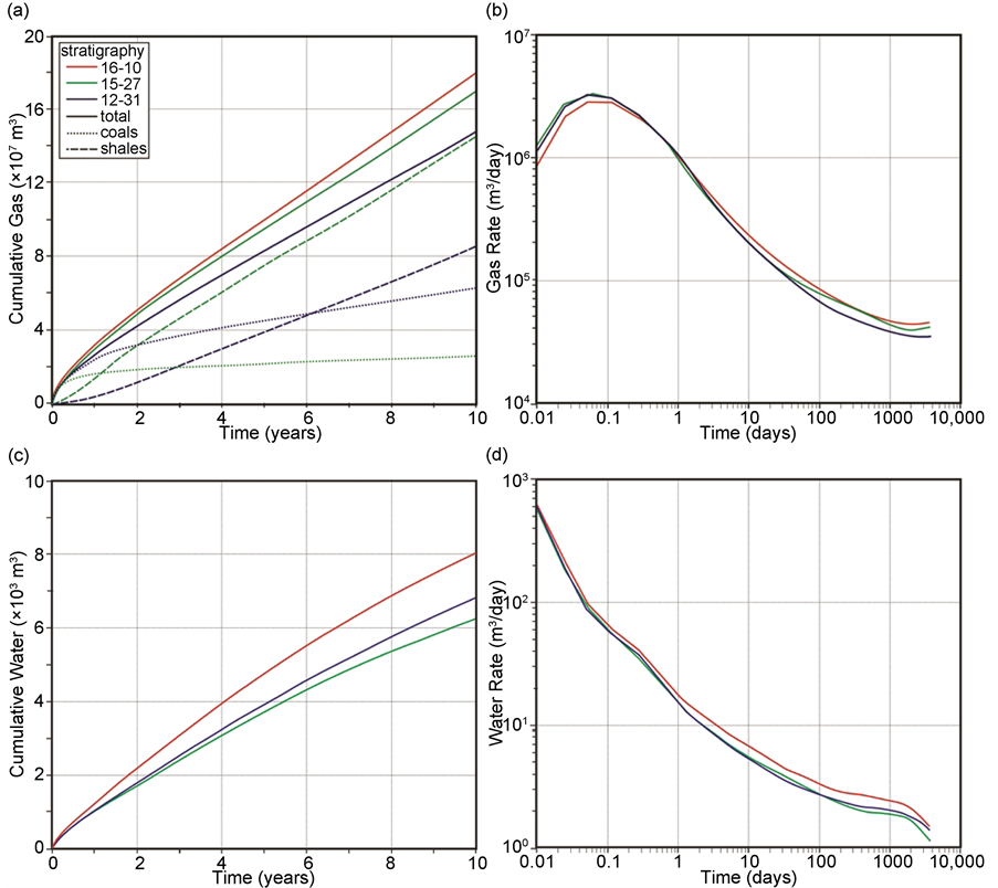
Figure 3. Comparison of the gas (top) and water (bottom) cumulative production (left) and production rates (right) simulated for the average model (16 - 10; red curves) versus models with the coal seam depths and thicknesses from the 12-31-61-06W5 well (12 - 31; blue curves) and 15-27-62-06W5 well (15 - 27; green curves). The recovered coal gas (dotted curves) versus recovered shale gas (dashed curves) is also shown for the end-member models on the cumulative gas production plot (a).
for the average model than the 15 - 27 model predicts 1.9× more produced water after 10 years of production, while the thicker main coal seam, and resulting greater volume of stored water in the fracture network, for the average model than the 12 - 31 model predicts 1.8× more produced water after 10 years of production (Figure 3(c)).
3.2. Coal Gas Content
The OGIP within the water-saturated Mannville Group is in the adsorbed state and the gas in productive area is almost entirely methane with a few percent of carbon dioxide ( [1] ). The statistical analysis of the Langmuir adsorption parameters determined from methane adsorption isotherm experiments provides the input values (Table 2). Increasing the adsorbed gas content of the coal seams, by changing the Langmuir constants (but keeping the initial reservoir pressure constant) between the P10 and P90 values, increases the coal OGIP by 2.3x. The higher coal OGIP has a decreasing impact on the gas producability with time, due to the longer required period of dewatering (due to higher initial gas saturations and thus lower relative permeability to water) as well as the decreasing importance of coal gas relative to shale gas (i.e. increasing ratio of recovered shale to coal gas with time) as the majority of the coal gas is produced during the early half of the production history, while the majority of the shale gas is produced during the latter half). The impact on the cumulative gas production due to varying the coal gas content from the P10 to P90 values decreases from 1.5× after 1 month of production to 1.1× after 10 years of production (Figure 4(a) and Figure 5(a)).
The higher gas saturations resulting from increased coal gas contents predicts
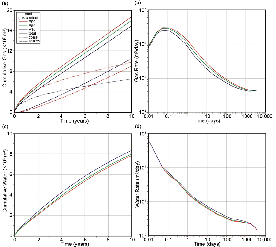
Figure 4. Comparison of the gas (top) and water (bottom) cumulative production (left) and production rates (right) simulated for the average model (VL = 13.7 cc/g and pL = 5.7 MPa; green curves) versus models with end-member coal adsorption capacities: maximum value of VL = 17.5 cc/g and pL = 3.8 MPa (red curves) and minimum value of VL = 9.9 cc/g and pL = 7.6 MPa (blue curves). The recovered coal gas (dotted curves) versus recovered shale gas (dashed curves) is also shown for the end-member models on the cumulative gas production plot (a).
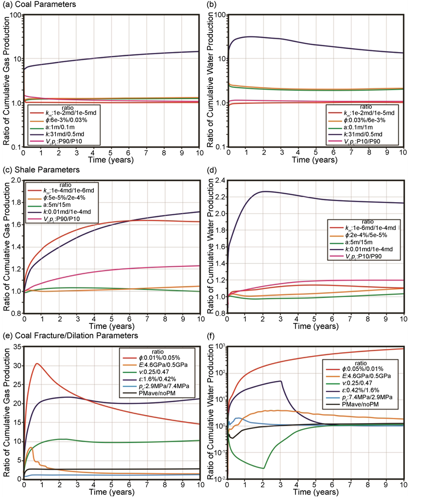
Figure 5. Comparison of the impact of the coal, shale, and coal fracture compaction/dilation parameters on the cumulative gas production (left) and the cumulative water production (right). The impact is calculated by the ratio of cumulative production between the end-member parameter values: (Top and Middle) Langmuir constants (VLpL; pink curve); matrix permeability (km; red curves), fracture porosity (f; orange curves), fracture spacing (a; green curves), and coal fracture permeability (k; blue curves); (Bottom) coal fracture porosity (f; red curves), coal Young’s modulus (E; orange curves), coal Poisson’s ratio (ν; green curves), coal maximum volumetric strain at infinite pressure (blue curves), and coal half-strain pressure (light blue curves). The ratios of the cumulative production between the model with the average coal fracture compaction/dilation parameters and the model with constant coal fracture permeability is also shown (black curves).
less water production, while the longer period of dewatering required by the higher gas saturations decreases the impact on the water production with time (Figure 4(b) and Figure 4(c)). Increasing the coal gas content between the end-member values results in 1.1× less produced water after 1 month of production and slightly (5.9%) less produced water after 10 years of production.
The higher cumulative gas production associated with higher coal gas contents results from the increased recovery of coal gas, whereas the recovery of shale gas decreases, due to the pressure maintenance of the coals. Increasing the coal gas content between the end-member values results in 1.5× more recovered coal gas after 10 years of production (dotted curves in Figure 4(a)) and 1.2× less recovered shale gas (dashed curves in Figure 4(a)). The importance of shale gas; therefore, decreases for higher coal OGIPs, resulting in a lower ratio of shale to coal gas (0.92 versus 1.6).
3.3. Coal Fracture Porosity
The Mannville coal has two well developed orthogonal cleats perpendicular to banding throughout the producing fairway; however, the in situ fracture aperture and hence the fracture porosity is poorly constrained as a result of dilation of the cleat with core recovery. Lacking physical measurements of the fracture porosity, a value has been estimated based on the match-stick model (ex. [11] [12] ). The match-stick model relates the average effective fracture spacing, fracture aperture width, initial fracture permeability, and fracture porosity. Therefore, the coal fracture porosity is recalculated when the coal fracture spacing and coal fracture permeability are varied during the parametric analysis. Increasing the coal fracture spacing from 0.1 m to 1 m, decreases the coal fracture porosity from 0.03% to 7× 10⁻³% and decreasing the coal fracture permeability from 31 md to 0.5 md, decreases the coal fracture porosity from 0.02% to 6× 10⁻³%.
Decreasing the coal fracture porosity from the maximum to minimum end-member values (from 0.03% to 6× 10⁻³%), which decreases the storage capacity of the fracture network for water (2.8× lower original-water-in-place, OWIP), results in a near-term higher relative permeability to gas and thus higher gas production and lower water production. Decreasing the coal fracture porosity between end-member values results in a 1.4× higher initial peak gas production rate (Figure 6(b)). The faster initial dewatering of the near wellbore region for smaller coal fracture porosities decreases the impact on the cumulative gas production to 1.2× after ~10 days of production (Figure 5(a) and Figure 6(a)). After which, the impact increases to 1.3× at the end of the 10 year production history as a result of the shorter required period of dewatering for smaller coal fracture porosities. Varying the coal fracture porosity between end-member values predicts 1.2× more coal gas and 1.4× more shale gas after 10 years of production (dotted and dashed curves in Figure 6(a)), resulting in a 1.1× higher ratio of recovered shale gas to coal gas (1.2 versus 1.0).
Varying the coal fracture porosity from the maximum to minimum end-member values results in 3.0× less produced water after 1 day of production, and the difference in produced water decreases to 2.1× after 5 years of production, due to the shorter period of dewatering required for smaller coal fracture
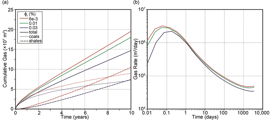
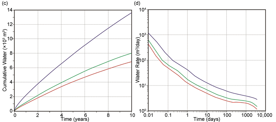
Figure 6. Comparison of the gas (top) and water (bottom) cumulative production (left) and production rates (right) simulated for the average model (0.01%; green curves) versus models with end-member coal fracture porosities: minimum value of 6 × 10⁻³% (red curves) and maximum value of 0.03% (blue curves). The recovered coal gas (dotted curves) versus recovered shale gas (dashed curves) is also shown for the end-member models on the cumulative gas production plot (a).
porosities (Figure 5(b) and Figure 6(c)). After 5 years, the impact of the coal fracture porosity on the cumulative water production slightly increases until the end of the 10 year period (difference of 2.1× after 10 years of production).
3.4. Coal Fracture Spacing
In reservoirs with low matrix permeability, the path length for gas transport through the matrix to the fracture network can limit the productivity. The path length is defined by the spacing between fractures that effectively transport gas. Although the Mannville coals have a well developed cleat system commonly spaced at less than 1 cm, the low system permeability indicates that most cleats must have no effective permeability to gas, either due to absence of fracture aperture due to high stress, or high compressibility of the coal matrix. The methods that exist for estimating the fracture spacing, which include geomechanical modelling, borehole image logs, and structural geometry, only provide a measure of the spacing between fractures that exist and not between effective fractures. Since we lack an accurate measure of the effective fracture spacing we have assumed an average effective fracture spacing of 0.50 m and end-member values of 0.1 m and 1 m in the coals.
Decreasing the coal effective fracture spacing between end-member values has a significant impact on the initial gas production rates (1.7× higher), but an insignificant impact on the cumulative gas production following the initial production period (0.040% difference after 10 years). However, the assumption of the applicability of the match-stick model leads to an increase in coal fracture porosity for decreasing coal fracture spacing. Decreasing the coal fracture spacing from the average value to the minimum end-member value increases the coal fracture porosity, resulting in a higher OWIP and a lower initial peak gas production rate. Whereas, increasing the coal fracture spacing from the average value to the maximum end-member value, results in a lower coal fracture porosity and OWIP and a higher initial peak gas production rate. Therefore, varying the coal fracture porosity with changes in the coal fracture spacing according to the match-stick model, predicts a smaller impact on the initial peak gas production rate than when the coal fracture porosity is held constant at the average value (1.2× versus 1.7x). Although decreasing the coal fracture spacing between end-member values results in a 1.2× higher initial peak gas production rate, the greater sensitivity of the producability to coal fracture porosity than coal fracture spacing, results in 1.3× less recovered gas after 10 years of production for a model with the smaller coal fracture spacing, but larger coal fracture porosity (Figure 5(a)). The larger coal fracture porosity for the minimum than the maximum end-member coal fracture spacing also results in 2.0× more produced water (Figure 5(b)) and a 1.1× lower ratio of recovered shale to coal gas after 10 years of production (1.0 versus 1.1).
3.5. Coal Fracture Permeability
The system permeability, which was obtained through pressure buildup testing of the Mannville coals at the well site, is approximated as the fracture permeability, due to the relatively much lower matrix permeability. The coal fracture permeability has the greatest impact on the producability of the Mannville reservoir of all the coal parameters. Increasing the coal fracture permeability from the minimum to maximum end-member values (0.5 md to 31 md), while holding the coal fracture porosity constant, results in 17× more produced gas and 8.0× more produced water after 10 years of production.
Higher coal fracture permeabilities are associated with higher coal fracture porosities and thus higher OWIPs. Including the assumption of the match-stick model; therefore, results in a smaller impact of the coal fracture permeability on gas production and a large impact on water production. Increasing the coal fracture permeability from the minimum to maximum end-member values, while also increasing the coal fracture porosity according to the match-stick model, predicts 14× more produced gas after 10 years of production (Figure 5(a) and Figure 7(a)). In addition to the faster drainage resulting from higher coal fracture permeabilities, the larger coal fracture porosity also predicts higher relative fracture permeability to water. Increasing the coal fracture permeability from the minimum to maximum end-member values predicts 31× more produced water after 1 year of production (Figure 5(b) and Figure 7(c)). The impact of the coal fracture permeability on water production decreases after ~1 year to 13× at the end of the 10 year production history, due to the shorter required period of dewatering.
Similarly to the other coal fabric parameters tested, the coal fracture permeability has a greater impact on the recovery of shale gas than coal gas. After 10 years of production, increasing the coal fracture permeability from the minimum
Figure 7. Comparison of the gas (top) and water (bottom) cumulative production (left) and production rates (right) simulated for the average model (3.8 md, 0.01%; green curves) versus models with end-member coal fracture permeabilities, when the coal fracture porosity is also changed according to the match-stick model: maximum value of 31 md (0.02%; red curves) and minimum value of 0.5 md (blue curves). The recovered coal gas (dotted curves) versus recovered shale gas (dashed curves) are also shown for the end-member models, on the cumulative gas production plot (a).
to maximum end-member values predicts 11× more produced coal gas (dotted curves in Figure 7(a)) and 19× more produced shale gas (dashed curves in Figure 7(a)), resulting in a 1.8× higher ratio of recovered shale to coal gas (1.4 versus 0.78).
Increasing the coal fracture permeability has a greater impact on increasing drainage from the main coal seam, where the lateral is placed, than the adjacent coal seams. The impact of increasing coal fracture permeabilities on increasing drainage from the minor coal seams decreases with distance from the wellbore. After 10 years of production, 13× more coal gas is recovered from the main coal seam for the maximum coal fracture permeability compared to 3.2× more from U1 (L1-12x; L2-10x; U2, U3-6.2x; U1-3.2x; Figure 8; see Figure 2(b) for location of seams). While the contribution from the main coal seam and L1 are higher for the maximum coal fracture permeability (1.1× higher for main coal seam and 4.9% higher for L1), the contributions from the other four coal seams are lower (U1-3.5x; U2, U3-1.8x; L2-1.1x; Table 3).
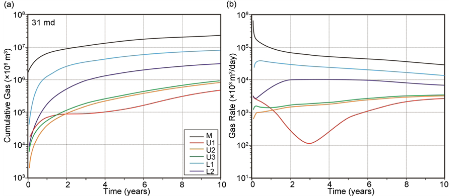
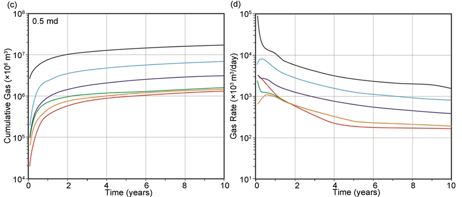
Figure 8. Comparison of cumulative gas recovered (left) and rate of gas recovery (right) from the main coal seam (M), the upper coal seams: U1 (red), U2 (orange), and U3 (green); and the lower coal seams: L1 (light blue) and L2 (blue) for a model with maximum (31 md; top) and minimum (0.5 md; bottom) end-member coal fracture permeabilities, when the coal fracture porosity is also changed according to the match-stick model.
Table 3. Contribution (in percentage) from coal seams to the produced coal gas for different lengths of production (in years).
3.6. Shale Gas Content
The statistical analysis of gas content data from desorbed shale samples has a P50 of 3.64 cc/g, which is significantly greater than the gas content calculated at the reservoir pressure from the average Langmuir parameters (0.85 cc/g; [6] ). Canister sampling is skewed towards carbonaceous (organic) rich samples, which have higher adsorption capacity, thus explaining the discrepancy between desorption and adsorption measurements. To provide a conservative estimate of the produced commingled shale gas, the average Langmuir parameters calculated from the adsorption data were input in the average model and the maximum and minimum values were input in the end-member models (Table 2).
Increasing the adsorbed gas content of the shale layers, by changing the Langmuir parameters from the average to maximum values has an insignificant impact on the producability of the Mannville reservoir (Figure 9(a)). At the depth of the S4 interbedded shale layer, the higher gas content for the maximum model results in a 2.9× higher OGIP than the average model; however, after 10 years, the cumulative gas production is only 0.13% higher (0.091% after 1 year).
In comparison, decreasing the adsorbed gas content of the shale layers between end-member values has a significant impact on the producability of the Mannville reservoir. While the initial production rate is not sensitive to the shale parameters (Figure 9(b)), as the production is initially restricted to the main coal seam, the lower relative permeability to gas, in addition to a 37× lower OGIP, for the minimum model delays gas recovery from the shales until after the first year of production (compared to after ~1 month of production for the maximum model; Figure 9(a)), resulting in 1.1× less produced gas after 1 year of production (Figure 5(c)). Although the maximum model requires a slightly longer period of dewatering than the minimum model (1860 vs 1700 days), the slower decline in gas production rates during dewatering and the faster increase in rates following dewatering increases the impact of the shale gas content on gas production to 1.2× after 10 years. The minimum model predicts 1.1× higher cumulative gas production after 10 years than a model with no adsorbed gas stored in the shales (Figure 9(a)). The higher relative permeability to gas associated with the higher shale OGIP for the maximum compared to the minimum shale gas content predicts l.2× less produced water after 10 years of production (Figure 5(c) and Figure 9(c)).
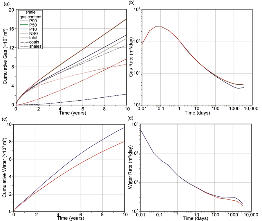
Figure 9. Comparison of the gas (top) and water (bottom) cumulative production (left) and production rates (right) simulated for the average model (VL = 1.5 cc/g and pL = 6.2 MPa ? green curves) versus models with end-member shale adsorption capacities: maximum value of VL = 7.2 cc/g and pL = 1.3 MPa (red curves) and minimum value of VL = 0.24 cc/g and pL = 11.4 MPa (blue curves). The recovered coal gas (dotted curves) versus recovered shale gas (dashed curves) are also shown for the end-member models on the cumulative gas production plot (a). The cumulative gas production for the model with gas-bearing coals, but no shale gas (NSG; grey curve) is also shown for comparison on plot (a). Note that the green curves for the average model (P50) are beneath the red curves for the maximum end-member model.
The increase in cumulative gas production predicted for larger shale gas contents results from increased shale gas recovery, while the coal gas recovery is reduced. After 10 years of production, 4.4× more shale gas (dashed curves in Figure 9(a)) and 1.5× less coal gas (dotted curves in Figure 9(a)) is predicted for the maximum shale gas content model than the minimum model, resulting in a 6.4× higher ratio of recovered shale to coal gas (1.1 versus 0.17).
3.7. Shale Matrix Permeability
The gas transport through the matrix of coals and shales is by the processes of diffusion and/or advection. Measuring the contribution from each process requires more sophisticated experiments than generally performed in the laboratory, carried out at a variety of pressures and/or multiple gases (i.e. [13] ). The matrix gas flux of the Mannville coal, calculated from experimental pulse decay data on crushed samples using the technique described in [13] are on the order of 10−3 md [14] . Shales generally have lower matrix gas transport rates than coals, thus a permeability of 1 × 10⁻⁵ md or equivalently a diffusion of 0.0008 cm2/s was chosen for the average model and values an order of magnitude higher and lower were chosen for the end-member models. The matrix permeability of the shales has a significant impact on the producability of the Mannville reservoir. While the initial production rate is not sensitive to the shale parameters, because the initial drawdown is restricted to the main coal seam near the wellbore, the maximum shale matrix permeability model predicts 1.6× more produced gas after 10 years of production than the minimum model (1 × 10⁻⁶ md to 1 × 10⁻⁴ md; Figure 5(c) and Figure 10(a)). The impact of shale matrix permeability on the cumulative gas production slightly decreases after ~7 years of production until the end of the 10 year production history as a result of the shorter period of dewatering and earlier increase in gas production rates for smaller shale matrix permeabilities, due to the lower gas saturations.
Increasing the shale matrix permeability by one order of magnitude from the average to maximum models results in 1.4× more produced gas after 10 years, whereas decreasing the shale matrix permeability by one order of magnitude from the average to minimum models results in 1.2× less produced gas after 10 years (Figure 10(a)). Note that the shale matrix permeability in the maximum model is only one order of magnitude lower than the average shale fracture permeability (1 × 10⁻⁴ vs 1 × 10⁻³ md). The gas in the maximum model can thus be efficiently transported through the matrix without travelling through the widely spaced fracture network (i.e. 10 m). The impact of the shale matrix permeability; however, is less important for smaller shale matrix permeabilities as there is a minimum gas production controlled by the coal fracture permeability. Therefore, decreasing the shale matrix permeability from 1 × 10⁻⁷ md to 1 × 10⁻⁸ md only has a slight impact on the produced gas (3.6% more for 1 × 10⁻⁷ md than 1 × 10⁻⁸ md; Figure 10(a)).
The lower gas saturations for the minimum shale matrix permeability results in 1.1× higher cumulative water production after 10 years of production history than the maximum value (Figure 5(d) and Figure 10(c)). The impact of the shale matrix permeability on the cumulative water production slightly decreases after ~5 years of production, due to the shorter period of dewatering for smaller shale matrix permeabilities. Similarly to the impact of the shale matrix permeability on the gas production, the impact of the shale matrix permeability on the water production is lower for smaller shale matrix permeabilities (ex. 3.8% difference between 1 × 10⁻⁷ md and 1 × 10⁻⁸ md; Figure 10(c)).
The higher produced gas predicted when increasing the shale matrix permeability between the end-member values results from 3.3× higher recovery of shale gas (dashed curves in Figure 10(a)), while the recovery of coal gas is 1.3× lower (dotted curves in Figure 10(a)). The ratio of recovered shale to coal gas; therefore, is 4.1× greater for the maximum than the minimum shale matrix permeabilities after 10 years of production (2.1 versus 0.50).
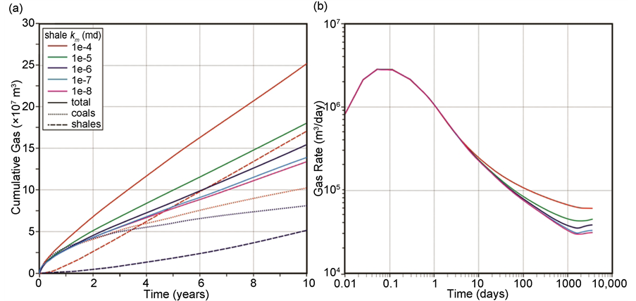
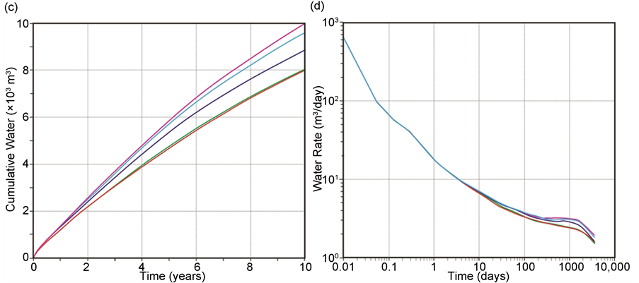
Figure 10. Comparison of the gas (top) and water (bottom) cumulative production (left) and production rates (right) simulated for the average model (1 × 10⁻⁵ md green curves) versus models with end-member shale matrix permeabilities: maximum value of 1 × 10⁻⁴ md (red curves) and minimum value of 1 × 10⁻⁶ md (blue curves); as well as models with shale matrix permeabilities of 1 × 10⁻⁷ md (light blue curves) and 1 × 10⁻⁸ md (pink curves). The recovered coal gas (dotted curves) versus recovered shale gas (dashed curves) are also shown for the end-member models on the cumulative gas production plot (a).
3.8. Shale Fracture Permeability
The fracture permeability for the Mannville shales has not been measured and a value of 0.001 md was estimated for the average model, based on measurements for gas shales of similar composition and diagenesis [15] and on a general understanding of gas shales. The values for the end-member models are an order of magnitude higher and lower than the assumed average value. Increasing the shale fracture permeability from the minimum to maximum end-member values (1 × 10⁻⁴ md to 0.01 md), while holding the coal fracture porosity constant at the average value, results in 1.9× more produced gas and 1.8× more produced water after 10 years of production.
Similarly to the coal fracture permeability, including the assumption of the match-stick model decreases the impact of the shale fracture permeability on gas production and increases the impact on water production. The impact of the shale fracture porosity decreases for smaller shale fracture permeabilities, due to the lower contribution from the shales to the gas production. Increasing the shale fracture permeability from the minimum to maximum end-member values, while also changing the shale fracture porosity according to the match-stick model, predicts 1.7× more produced gas after 10 years of production (Figure 5(c) and Figure 11(a)) and a maximum of 2.3× less produced water after ~2 years of production (Figure 5(d) and Figure 11(c)). The faster dewatering for larger shale fracture permeabilities decreases the impact on cumulative water production from the maximum to 2.1× after 10 years of production. The higher gas production predicted for the maximum than the minimum shale fracture
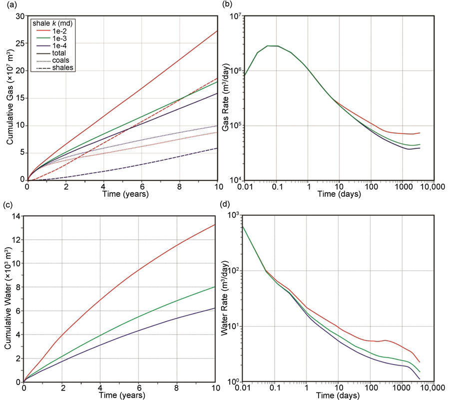
Figure 11. Comparison of the gas (top) and water (bottom) cumulative production (left) and production rates (right) simulated for the average model (1 × 10⁻³ md, 1 × 10⁻⁴%; green curves) versus models with end-member shale fracture permeabilities, when the shale fracture porosity is also changed according to the match-stick model: maximum value of 1 × 10⁻² md (2 × 10⁻⁴%; red curves) and minimum value of 1 × 10⁻⁴ md (5 × 10⁻⁵%; blue curves). The recovered coal gas (dotted curves) versus recovered shale gas (dashed curves) are also shown for the end-member models, with varying coal fracture porosity, on the cumulative gas production plot (a).
permeabilities results from a 3.1× greater recovery of shale gas (dashed curves in Figure 11(a)), while the recovery of coal gas is 1.1× lower (dotted curves in Figure 11(a)), resulting in a 3.5× higher ratio of shale to coal gas recovered after 10 years of production (2.1 versus 0.60).
3.9. Stress-Dependent Coal Fracture Permeability
The fracture permeability in coal and shale reservoirs can vary strongly with effective stress. The drawdown in fluid pressure accompanying production results in an increase in effective stress, which can reduce the fracture permeability, the amount of which depends on the rock mechanical properties and fabric of the reservoir. The decrease in permeability may be offset by matrix shrinkage due to methane desorption during production, which depending on the sorption-in duced volumetric strain, enhances the fracture permeability and potentially causes the permeability to rebound. Several analytical models are available for predicting the stress-dependent fracture permeability of coal seams during production ( [5] [16] [17] [18] ). As part of the parametric analysis, the Palmer-Manssori model [5] , which is incorporated in the GEM simulator, is used to investigate the variability in productivity with changes in the coal seam Young’s modulus (E), Poisson’s ratio (ν), average half-strain pressure ( ), and maximum strain at infinite pressure (ε) (Table 2). The equation for the permeability multiplier (k/k0) used by the simulator to calculate the stress-dependent fracture permeability depends on the change in pressure (
 ) according to:
 (1)
(1)
where:
 (2)
(2)
 (3)
(3)
 and (4)
 (5)
(5)
which was modified by CMG from the original Palmer-Mansoori model to avoid negative porosity values.
Although some rock mechanics data are available for the organic rich shales interbedded with the Mannville coal seams, the long test-times (up to a year), due to the very low matrix permeability of shales, has hindered laboratory sorption-induced strain experiments, and thus the dynamic changes in shale fracture permeability are poorly understood. The fracture permeability for the shales was thus held constant during the modeling.
3.9.1. The Average Stress-Dependent Coal Fracture Permeability Model
Including the coal fracture compaction/dilation parameters, with the average parameter values listed in Table 2, in the model to predict the dynamic changes in the coal fracture permeability during simulation increases the cumulative gas production by 31× after 10 years of production (0.01% models in Figure 12(a)) and decreases the water production by 317× (Figure 12(c)). The dilation of the coal fractures, due to matrix shrinkage with gas desorption, increases the maximum coal fracture permeability by up to 17 D (i.e. 1.7 × 10⁴ md) over the 10 year production history. The coal fracture porosity estimated from the match-stick
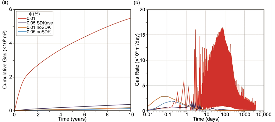
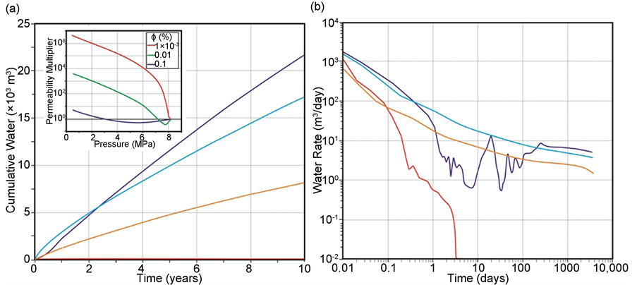
Figure 12. Comparison of the gas (top) and water (bottom) cumulative production (left) and production rates (right) simulated for the constant coal fracture permeability model with average coal fracture porosity of 0.01% calculated from the average effective coal fracture spacing (0.50 m) using the match-stick model (0.01% noSDK ? orange curves) and the stress-dependent coal fracture permeability model with the coal fracture porosity of 0.01% (0.01% ? red curves). The production histories for the constant coal fracture permeability model with coal fracture porosity calculated from the observed average coal cleat spacing (0.05 m) using the match-stick model (0.05% noSDK ? light blue curves) and the stress-dependent coal fracture permeability model with the coal fracture porosity of 0.05% (0.05% SDKave ? blue curves) are also plotted. The inset plot in (c) shows the change in the fracture permeability multiplier with pressure calculated from the modified Palmer-Mansoori equation used in the GEM simulator for fracture porosities of 0.1, 0.01 and 1 × 10⁻³%.
model; therefore, predicts an unrealistic increase in the coal fracture permeability. The fracture porosity was calculated assuming the effective fracture spacing; however, a fracture may have significant yet disconnected porosity. A true coal cleat spacing, an order of magnitude smaller than the effective fracture spacing (from 0.5 m to 0.05 m) was used to calculate the coal fracture porosity (0.05%), which was held constant while varying the other coal fracture dilation/compact- tion parameters.
A stress-dependent coal fracture permeability model with a coal fracture porosity of 0.05% predicts 2.8× more produced gas than a constant coal fracture permeability model with a coal fracture porosity of 0.05% after 10 years of production (Figure 5(e) and Figure 12(a)) and 1.9× more produced water (Figure 5(f) and Figure 12(c)). The matrix strain due to increasing effective stress decreases the permeability by up to 2.3 md, while the matrix shrinkage then increases the maximum coal fracture permeability by up to 140 md. Although the initial peak gas production rate is 2.5× lower (Figure 12(b)) as a result of matrix strain and the reduction of coal fracture permeabilities near the wellbore, the rebound of the coal fracture permeabilities with matrix shrinkage predicts 1.9× higher cumulative gas production after 1 month of production. The impact of the dynamic changes in coal fracture permeability slightly increases from 1 month until the end of the 10 year production history.
The trade-off between coal fracture dilation and compaction result in undulating production rates (Figure 12(b) and Figure 12(d)). Once the fracture permeability in the coals near the wellbore rebounds, the fracture permeability decreases in the coals farther from the wellbore, which increases the drainage from the coals near the wellbore. The fracture permeability in the coals farther from the wellbore rebounds with continued production, which decreases the pressure in the coals near the wellbore thus decreasing the fracture permeability.
The enhanced coal fracture permeability with matrix shrinkage predicts 2.8× higher coal gas recovery (solid curves in Figure 13(a)) and 2.9× higher shale gas recovery (dotted curves in Figure 13(a)) resulting in a slightly higher ratio of recovered shale to coal gas than the constant fracture permeability model (1.0 versus 0.97 after 10 years of production). While the enhanced permeability increases drainage throughout the reservoir, the impact decreases with distance from the wellbore. After 10 years of production, the enhanced coal fracture permeability predicts 3.0× higher gas recovery from the main coal seam compared to 1.5× from U1 (L1-2.7×; L2-2.4×; U2, U3-2.0×; Figure 14(a) and Figure 14(c)). The enhanced permeability in the stress-dependent permeability model compared to the constant permeability model increases the contribution of the recovered gas from the main coal seams and decreases the contribution of the recovery gas from the minor coal seams (Table 4).
3.9.2. Coal Fracture Porosity
Smaller fracture porosities predict a rebound in the coal fracture permeability at higher pressures (i.e. shorter production time) and a larger increase in fracture permeability, due to matrix shrinkage (inset plot in Figure 12(c)). While a model
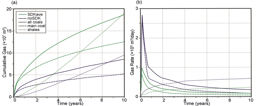
Figure 13. Comparison of cumulative gas recovered (left) and rate of gas recovery (right) from all the coal seams (solid curves), only the Mannville coal seam (dashed curves), and the shale layers (dotted curves) for the average stress-dependent coal fracture permeability model (SDKave―green curves) and for the constant coal fracture permeability model (noSDK―blue curves).
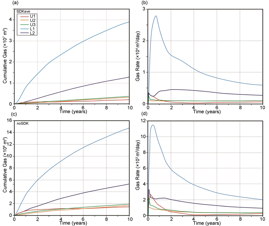
Figure 14. Comparison of cumulative gas recovered (left) and rate of gas recovery (right) from the upper coal seams: U1 (red), U2 (orange), and U3 (green); and the lower coal seams: L1 (light blue) and L2 (blue) for the average stress-dependent coal fracture permeability model (SDKave―top) and for the constant coal fracture permeability model (noSDK―bottom).
Table 4. Contribution (in percentage) from coal seams to the produced coal gas for different lengths of production (in years).
with the average coal fracture porosity (0.05%) predicts a maximum coal fracture permeability of 1.4 × 10² md and a minimum coal fracture permeability of 1.7 md, a model with a smaller coal fracture porosity (0.01%) predicts a coal fracture permeability of 1.7 × 10⁴ md over the 10 year production history. The smaller coal fracture porosity model predicts a maximum of 30× more produced gas after ~9 months of production than the average model (0.05%; Figure 5(e) and Figure 12(a)). The impact of the coal fracture porosity then decreases to 15× at the end of the 10 year production history as a result of the faster reservoir depletion for smaller coal fracture porosities. The higher cumulative gas production predicted for the smaller coal fracture porosity results from 17× more produced shale gas and 12× more produced coal gas, resulting in a higher ratio of the recovered shale to coal gas (1.4 versus 1.0 after 10 years of production). The initial water production rate for the smaller coal fracture porosity model is 1.5× lower than the average model (Figure 12(d)) as a result of the higher gas saturations and ceases after 25 m3 have been produced, a volume 88× less than the cumulative water production for the average model after 1 year and 8.6 × 10²× less after 10 years (Figure 5(f) and Figure 12(c)).
3.9.3. Coal Young’s Modulus
The matrix shrinkage is independent of the Young’s modulus; however, the Young’s modulus has a significant impact on the matrix dilation due to increasing effective stress during production. Stiffer rocks with larger Young’s moduli, induce smaller strains for the same change in stress, resulting in smaller decreases in fracture permeability with increasing effective stress (inset plot of Figure 15(c)). Therefore, while a model with the maximum coal Young’s modulus (4.6 GPa) predicts enhanced fracture permeability in the main coal seam surrounding the wellbore from the onset of production, a model with the minimum coal Young’s modulus (0.5 GPa) initially predicts a large reduction in permeability. Both models predict a large increase in fracture permeability in the main coal seam near the wellbore later in the production history (by up to 1.5 × 10² md for the maximum model compared to 1.4 × 10² md for the minimum model), while the fracture permeability farther from the wellbore decreases, due to matrix strain, (by up to 0.52 md in the maximum model compared to 3.9 md in the minimum model).

Figure 15. Comparison of the gas (top) and water (bottom) cumulative production (left) and production rates (right) simulated for the average stress-dependent coal fracture permeability model (2.3 GPa―green curves) versus models with end-member coal Young’s modulus: maximum value of 4.6 GPa (red curves) and minimum value of 0.5 GPa (blue curves). The cumulative gas and water production for the constant coal fracture permeability model are also shown (noSDK―green dashed curves). The inset plot in (c) shows the change in the fracture permeability multiplier with pressure calculated from the modified Palmer-Mansoori equation used in the GEM simulator for coal Young’s modulii of 0.5, 2.3, and 4.6 GPa.
The initial increase in fracture permeability in the main coal seam surrounding the wellbore for the maximum model and the initial decrease in fracture permeability for the minimum model results in a 4.1× higher initial gas production peak for the maximum than the minimum models (Figure 15(b)). The impact of the coal Young’s modulus (Figure 5(e)) increases to a maximum of 16× after ~3 days of production, due to the greater reduction in coal fracture permeability with matrix strain for smaller coal Young’s moduli. The delayed fracture permeability rebound for smaller coal Young’s moduli decreases the impact of the coal Young’s modulus on the cumulative gas production to 3.8× after 1 year of production and 1.5× after 10 years of production. The shale gas recovery is 1.8× higher and the coal gas recovery is 1.3× higher for the model with the maximum coal Young’s modulus, resulting in a 1.3× higher ratio of shale to coal gas than the model with the minimum coal Young’s modulus after 10 years of production (ratio of 1.1 versus 0.84). While the model with the larger coal Young’s modulus initially predicts a lower water production rate (Figure 15(d)), the cumulative water production is 3.8× higher after ~2 years of production and 1.9× higher at the end of the 10 year period (Figure 5(f) and Figure 15(c)).
3.9.4. Coal Poisson’s Ratio
A larger Poisson’s ratio implies a larger pore volume modulus, which induces smaller reductions in the pore volume of rock thus resulting in smaller reductions in coal fracture permeability with increasing effective stress (inset plot of Figure 16(c)). The Poisson’s ratio also has a significant impact on the matrix shrinkage with gas desorption. Smaller Poisson’s ratios result in earlier fracture
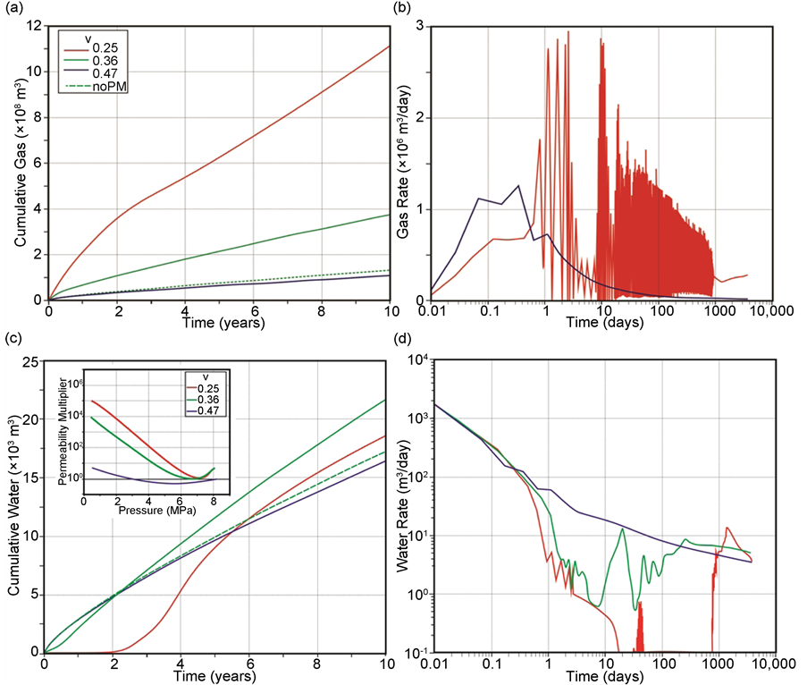
Figure 16. Comparison of the gas (top) and water (bottom) cumulative production (left) and production rates (right) simulated for the average stress-dependent coal fracture permeability model (0.36―green curves) versus models with end-member coal Poisson’s ratios: maximum value of 0.25 (red curves) and minimum value of 0.47 (blue curves). The cumulative gas and water production for the constant coal fracture permeability model are also shown (noSDK―green dashed curves). The inset plot in (c) shows the change in the fracture permeability multiplier with pressure calculated from the modified Palmer-Mansoori equation used in the GEM simulator for coal Poisson’s ratios of 0.25, 0.36, and 0.47.
permeability rebounds and greater increases in fracture permeability with matrix shrinkage. Therefore, smaller coal Poisson’s ratios induce a much large range of coal fracture permeabilities (1.7 × 10² - 4.8 × 10² md for the minimum coal Poisson’s ratio of 0.25 compared to 2.1 - 5.7 md for the maximum coal Poisson’s ratio of 0.47).
The greater reduction in fracture permeability, due to matrix swelling, for the smaller coal Poisson’s ratios results in a 1.6× lower initial peak gas production rate (Figure 16(b)).
However, the earlier coal fracture permeability rebound and greater matrix shrinkage for the minimum coal Poisson’s ratio, delays dewatering until ~2 years of production, while the lower matrix shrinkage predicted for the maximum coal Poisson’s ratio results in continuously declining gas production rates over the 10 year production history. The minimum model thus predicts a maximum of 11× more produced gas and 38× less produced water after ~2 years of production (Figure 5(e) and Figure 5(f) and Figure 16(a) and Figure 16(c)). After which, the impact of the coal Poisson’s ratio on gas production decreases to 9.8× after ~5 years of production, during dewatering for the minimum coal Poisson’s ratio, and then following dewatering, the impact increases to 10× at the end of the 10 year period. The shale gas recovery for the minimum model is 12× higher and the coal gas recovery is 8.8× higher, resulting in a 1.4× higher ratio of recovery shale to coal gas than the maximum model after 10 years of production (1.2 versus 0.87). The influx of water from the enhanced fracture permeability in the coals farther from the wellbore, following dewatering for the minimum model, results in greater cumulative water production after ~5.5 years of production and a maximum of 1.1× more produced water after ~9.5 years of production, following which the impact on cumulative water production slightly decreases as a result of the faster dewatering for the minimum model.
3.9.5. Coal Maximum Volumetric Strain at Infinite Pressure
While the maximum volumetric strain at infinite pressure has no influence on the matrix swelling, larger coefficients induce greater matrix shrinkage resulting in earlier fracture permeability rebound and a greater increase in fracture permeability with matrix shrinkage (inset plot in Figure 17(c)). Therefore, the maximum end-member value for the coal max strain (1.6%) predicts smaller reductions in fracture permeability (1.2 md versus 3.6 md) and larger increases in coal fracture permeability (5.4 × 10² md versus 6.1 md) than the minimum end-member value (0.47%).
The earlier coal fracture permeability rebound and greater matrix shrinkage for larger coefficients, delays dewatering for the maximum model until ~3 years of production, while the greater reduction in coal fracture permeability for the minimum model results in a lower initial peak gas production rate and continuously declining gas production rates over the 10 year period (Figure 17(b)). Thus, the maximum model predicts a maximum of 22× more produced gas and 51× less produced water than the minimum model after ~3 years of production (Figure 5(e) and Figure 5(f) and Figure 17(a) and Figure 17(c)). After which,
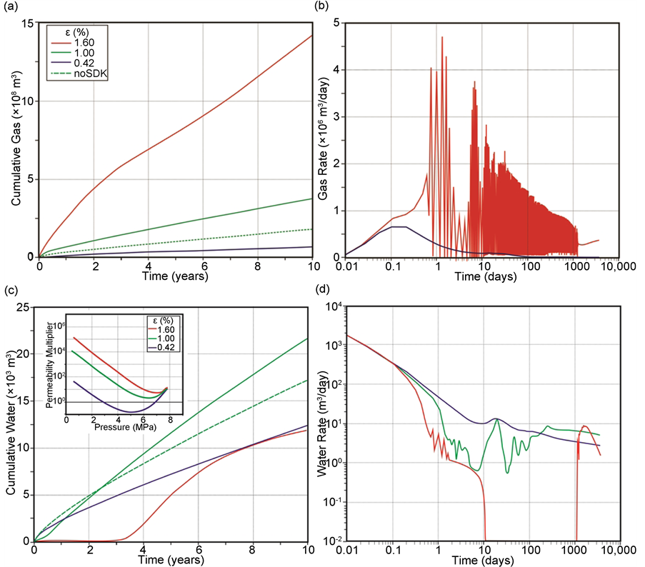
Figure 17. Comparison of the gas (top) and water (bottom) cumulative production (left) and production rates (right) simulated for the average stress-dependent coal fracture permeability model (1.00%―green curves) versus models with end-member coal maximum volumetric strain at infinite pressure: maximum value of 1.60% (red curves) and minimum value of 0.42% (blue curves). The cumulative gas and water production for the constant coal fracture permeability model are also shown (noSDK―green dashed curves). The inset plot in (c) shows the change in the fracture permeability multiplier with pressure calculated from the modified Palmer-Mansoori equation used in the GEM simulator for coal maximum volumetric strains at infinite pressure of 0.42%, 1.00% and 1.60%.
the impact of the coefficient decreases to 20× after ~5.5 years of production, during dewatering for the maximum model, and then increases following dewatering to 21× at the end of the 10 year production history. The recovered shale gas is 31× higher and the recovered coal gas is 15× higher for the maximum model, resulting in a 2.0× higher ratio of recovered shale to coal gas than the minimum model (ratio of 1.2 versus 0.61). The influx of water from the enhanced fracture permeability in the coals farther from the wellbore, following dewatering for the larger coefficient, results in a minimum of 0.85% less produced water after ~8 years of production, following which the impact on cumulative water production slightly decreases as a result of the faster dewatering for the maximum model (4.6% less produced water for maximum model after 10 year period).
4. Discussion and Conclusions
The Mannville coal measures of the Western Canadian Sedimentary Basin are a complex reservoir in which production from horizontal wells drilled and completed in the thickest coal seam in the succession (~1 m versus 3 m) has production and pressure support from thinner coals in the adjacent stratigraphy and from organic-rich shales interbedded and over and underlying the coal seams. The results from a series of numerical simulations are summarized and discussed to investigate the impact of gas content and fabric parameters on the producability of the gas stored within the minor coal seams and shale beds. The goal of the modeling is to quantify and rank the importance of the coal and shale parameters through a parametric analysis. The input parameters for the modelling were obtained through a statistical analysis of laboratory and field data compiled from industry and academic databases as well as from new laboratory tests.
The impacts of the model parameters, which were quantified during a parametric analysis as the ratio (or percent difference if ratio < 1.1x) of models with end-member values, on the cumulative gas and water production, as well as on the ratio of produced shale to coal gas after 10 years of production are compared in Table 5 and Figure 18. The results for varying coal and shale parameters with constant coal fracture permeability are first presented in order of decreasing
Table 5. Comparison of the impact of the model parameters after 10 years of production. The impacts were quantified as the ratio (or percent difference if ratio < 1.1) of models with end-member values.
k-fracture permeability; km-matrix permeability; f-fracture porosity; a-fracture spacing; VLpL-Langmuir constants; SDK-stress-dependent coal k; ε-maximum volumetric strain; E-Young’s modulus; ν-Poisson’s ratio; pε-half-strain pressure.
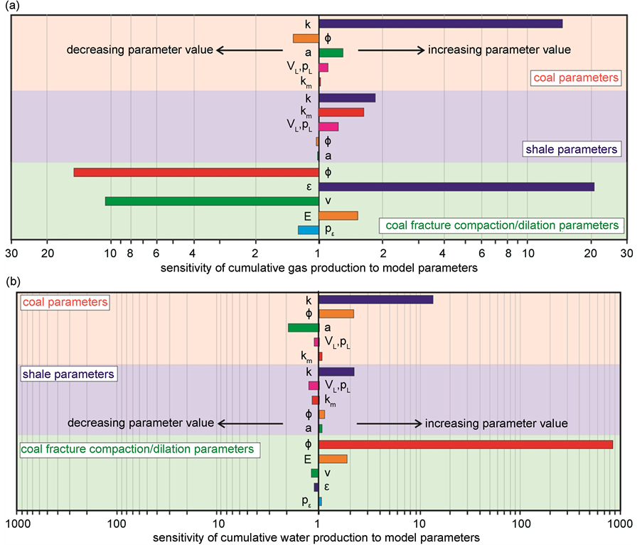
Figure 18. Comparison of the sensitivity of the cumulative gas (a) and water (b) production after 10 years of production to the coal parameters (red boxes), shale parameters (blue boxes), and coal fracture compaction/dilation parameters (green boxes) in order from most to least sensitive. The sensitivity is quantified as the ratio of the cumulative production for the end-member parameter values. Increased cumulative production resulting from the increase in model parameters from minimum to maximum end-member values are plotted on the right and increased cumulative production resulting from the decrease in model parameters from maximum to minimum end-member values are plotted on the left. k-fracture permeability; km-matrix permeability; f-fracture porosity; a-fracture spacing; VLpL-Langmuir constants; ε-maximum volumetric strain; E-Young’s modulus; ν-Poisson’s ratio; pε-half-strain pressure.
impact. The results for varying coal fracture compaction/dilation parameters are then compared (Table 5 and Figure 18).
4.1. Impact of Coal and Shale Parameters
The simulation results for a model with gas-bearing coal and shale layers predict that the cumulative gas production from a single 1000 m long lateral in the main Mannville coal seam increases by a maximum of 14× at the end of a 10 year history when the coal fracture permeability (k) is increased from the minimum to the maximum end-member values (0.05 to 31 md), while holding all the other model parameters constant at their average values and ignoring dynamic changes in permeability with production (blue bar in red box in Figure 18(a)). In comparison, the model parameter with the next greatest impact on the gas production is the shale k, which when increased between end-member values (1 × 10⁻⁴ and 0.01 md) increases the cumulative gas production by a maximum of 1.7× at the end of the 10 year period (blue bar in blue box in Figure 18(a)). The impact of increasing the shale matrix permeability (km; 1 × 10⁻⁷ and 1 × 10⁻³; red bar in blue box in Figure 18(a)) is lower than the impact of increasing shale k at the end of the 10 year production history (1.6x); however, the impact is greater until ~6 years of production.
Lacking physical measurements, the coal fracture porosity (f) was estimated during this study based on the match-stick model, which relates the fracture spacing, porosity, and permeability. Decreasing coal f (0.03% to 6 × 10⁻³%), which decreases the storage capacity of the fracture network for water, predicts a maximum of 1.3× higher cumulative gas production at the end of the 10 year production history (orange bar in red box in Figure 18(a)). The coal f, which is the coal parameter with the second greatest impact on the gas production after coal k, initially has a greater impact than the shale matrix and fracture permeabilities (until ~4 months and ~9 months). The coal parameter with the least impact on the cumulative gas production is the coal fracture spacing (a; 1 and 0.01 m; 0.040% after 10 years); however, the associated changes in the coal f result in a similar impact as the coal f over the 10 year production history (1.3× after 10 years; green bar in red box in Figure 18(a)). The model parameter with the next greatest impact on the gas production is the shale gas content (VLpL), which increases the cumulative gas production by a maximum of 1.2× at the end of the 10 year history when increased between end-member values (0.24 cc/g, 1.3 MPa and 7.2 cc/g, 11.4 MPa; pink bar in blue box in Figure 18(a)). Whereas, shale VLpL has a greater impact than coal VLpL at the end of the 10 year production history (1.1× after 10 years; 9.9 cc/g, 3.8 MPa and 17.5cc/g, 7.6 MPa; pink bar in red box in Figure 18(a)), the impact is lower until ~4 years of production. The impact of coal VLpL on the early cumulative gas production is also greater than the impacts of coal f and coal a until ~1.5 years of production.
4.1.1. Water Production
Increasing coal k and shale k results in higher gas, as well as higher water production (Figure 18(b)). In contrast, increasing the cumulative gas production by varying the other model parameters decreases the cumulative water production (Figure 18(b)). The cumulative water production is most sensitive to variations in coal k, which predicts a difference of 13× after 10 years (blue bar in red box in Figure 18(b)). In comparison, the coal f, which has the next greatest impact on the water production, predicts a difference of 2.1× after 10 years (orange bar in red box in Figure 18(b)). The shale k (2.1× after 10 years; blue bar in blue box in Figure 18(b)) is the shale parameter with the largest impact on the cumulative water production and while the impact is slightly lower than for coal f at the end of the 10 year history, the impact is greater from ~1.5 - 9.5 years of production. The coal a (2.0× after 10 years; green bar in red box in Figure 18(b)), which initially has a higher impact than shale k (until ~1 years) has the next greatest impact on the cumulative water production. The shale VLpL (1.2× after 10 years; pink bar in blue box in Figure 18(b)), which is the shale parameter with the next greatest impact on the water production after the shale k, has a greater impact on the cumulative water production than the coal VLpL after ~2.25 years of production. The coal VLpL (6% after 10 years; pink bar in red box in Figure 18(b)) is also initially greater than the impact of the shale km (until ~3 years; 1.1× after 10 years; red bar in blue box in Figure 18(b)).
4.1.2. Produced Coal Gas versus Shale Gas
The importance of shale gas increases for more favourable shale parameters resulting in higher ratios of recovered shale to coal gas. The higher cumulative gas production for more favourable shale parameters results from the increased recovery of shale gas, while the recovery of coal gas is reduced for all shale parameters (with the exception of shale f). Such results indicate that once the easily accessible coal gas has been recovered, the shale gas is preferentially recovered resulting in the lower coal gas recovery for favourable shale parameters. The importance of shale gas also increases for more favourable coal fabric parameters, resulting in a higher ratio of recovered shale to coal gas, whereas the importance of shale gas decreases for higher coal gas contents, resulting in a lower ratio of recovered shale to coal gas. The maximum shale permeabilities predict the highest ratios of recovered shale to coal gas (2.1 after 10 years), while the minimum shale VLpL predicts the lowest (0.17 after years). Variations in shale VLpL have the greatest impact on the ratio of recovered shale to coal gas of all the parameters (1.1 versus 0.17; 6.4× after 10 years), followed by shale km (2.1 versus 0.50; 4.1× after 10 years), then shale k (2.1 versus 0.60; 3.5× after 10 years). The coal parameters have lower impacts on the ratio of recovered shale to coal gas compared to the shale parameters. The coal parameters with the greatest impact on the ratio of recovered shale to coal gas are coal k (1.4 versus 0.78; 1.8× after 10 years) and coal VLpL (0.92 versus 1.6; 1.7× after 10 years), followed by coal f and coal a (both 1.1× after 10 years).
4.2. Impact of Coal Fracture Dilation/Compaction Parameters
The variation in coal k with effective stress and matrix shrinkage due to production predicts 2.8× more produced gas, 1.9× more produced water, and a slightly higher ratio of recovered shale to coal gas (3.0% after 10 years) than for a constant coal k after 10 years of production. The dynamic changes in coal k and the resulting impact on producability are very sensitive to variations in the coal fracture dilation/compaction parameters. Varying coal f has the greatest impact on the dynamic changes in coal k during production, resulting in the greatest change in the cumulative gas production (30× at 9 month). The coal maximum volumetric strain (ε; 21x; blue bar in green box in Figure 18(a)); however, has a greater impact on the cumulative gas production than coal f (15× after 10 years; red bar in green box in Figure 18(a)) after ~3.5 years of production. The impact of varying a constant coal k (i.e. when dynamic changes with production are ignored; 14× after 10 years; blue bar in red box in Figure 18(a)), are lower than the impacts of coal ε and coal f, while greater for most or all of the 10 year history than the impacts of the coal Poisson’s ratio (ν; lower from ~0.5 - 2 years) and coal Young’s modulus (E; lower from ~4 - 6 months). The coal E (1.5× after 10 years; orange bar in green box in Figure 18(a)) has a greater impact on the cumulative gas production than coal ν (10× after 10 years; green bar in green box in Figure 18(a)) until ~6 months of production; however, has a much lower impact than coal ν at the end of the production history. The impact of coal E is also lower than the impacts of shale k and shale km after ~6 years of production.
4.2.1. Water Production
The large matrix shrinkage predicted for smaller coal f, which results in higher cumulative gas production, ceases water production following the initial drawdown. Decreasing the coal f, for stress-dependent coal k, thus results in much lower cumulative water production and a much greater impact on the cumulative water production than the other model parameters (8.6 × 10²× after 10 years; red bar in green box in Figure 18(b)). The large matrix shrinkage predicted for large coal ε and small coal ν delays the water production resulting in a peak impact on the cumulative water production early in the production history (51× after ~3 years for coal ε; 38× after ~2 years for coal ν). The enhanced permeability decreases the impacts following the peaks and while the cumulative water production for the maximum coal ε remains lower, the cumulative water production is higher for the minimum coal ν after ~5.5 years of production. The enhanced coal k for the maximum coal E results in higher cumulative gas and water production over the majority of the 10 year production history, although the smaller matrix swelling results in lower cumulative water production until ~4 months of production.
After 10 years of production, coal E (1.9× after 10 years; orange bar in green box in Figure 18(b)) is the coal fracture compaction/dilation parameter with the next greatest impact on cumulative water production, after coal f. However, the large impacts of coal ε (4.6% after 10 years; blue bar in green box in Figure 18(b)) and coal ν (1.1× after 10 years; green bar in green box in Figure 18(b)) on the early cumulative water production are greater than the impact of coal E as well as all the coal and shale parameters. The impact of coal ε decreases and remains lower than all the model parameters and the impact of ν also decreases lower than the impacts of the other model parameters with the exception of coal VLpL and shale km.
4.2.2. Produced Coal Gas versus Shale Gas
Increasing the cumulative gas production by varying the coal fracture compaction/dilation parameters, similarly to varying a constant coal k (i.e. assuming no dynamics changes), results in a greater ratio of recovered shale to coal gas. The impact of coal ε (2.0× after 10 years) on the ratio of recovered shale to coal gas, which is greater than the other coal fracture compaction/dilation parameters, is also greater than all the coal parameters. In contrast, the other coal fracture compaction/dilation parameters have lower impacts on the ratio of recovered shale to coal gas than coal VLpL and constant coal k. The impacts of coal f and coal ν are approximately the same (both 1.4 after 10 years, although impact of coal ν is very slightly greater) and slightly greater than the impact of coal E (1.3× after 10 years).
4.3. Conclusions
The results of the parametric analysis predict that the coal fracture permeability has the greatest impact on the cumulative gas and water production, when dynamic changes with production are ignored. At the end of 10 years of production, 14× more gas and 13× more water is predicted when the coal fracture permeability is increased between end-member values (0.5 md and 31 md). In comparison, the parameters with the next greatest impacts on the gas production are the fracture and matrix permeabilities of adjacent organic rich shales. After 10 years, an increase in shale fracture permeability from end member values of 1 × 10⁻⁴ and 0.01 md predicts an increase in production of 1.7× and an increase in shale matrix permeability from 1 × 10⁻⁷ to 1 × 10⁻³ md predicts an increase in production of 1.6×. The coal and shale fracture permeabilities are the only parameters that result in increased water production when the gas production increased. The parameters with the greatest impacts on the cumulative water production evaluated after 10 years of production. Following coal fracture permeability are coal fracture porosity (2.1x), shale fracture permeability (2.1x), and coal fracture porosity (2.0x).
Organic rich shales over and underlying the completed coal seams contribute significantly to the total gas produced. The relative contribution of shale gas to total gas varies with the shale and coal storage and properties. The higher cumulative gas production for more favourable shale parameters (with the exception of shale fracture porosity) is due to greater recovery of gas from the shales. While less coal gas is recovered, resulting in higher ratios of recovered shale to coal gas. More favourable coal fabric parameters predict greater recovery from both the shales F and the coals, also resulting in higher ratios of recovered shale to coal gas; however, with a lower impact than the shale parameters. Whereas, increasing the coal gas content predicts greater coal gas recovery and lower shale gas recovery resulting in a lower ratio. The maximum shale permeabilities predict the highest ratios of recovered shale to coal gas (2.1 after 10 years), while the minimum shale gas content predicts the lowest (0.17 after years). Variations in shale gas content have the greatest impact on the ratio of recovered shale to coal gas of all the parameters (1.1 versus 0.17 after 10 years), followed by shale matrix permeability (2.1 versus 0.50 after 10 years), then shale fracture permaeability (2.1 versus 0.60 after 10 years). The coal parameters with the greatest impact on the ratio of recovered shale to coal gas are coal fracture permeability (1.4 versus 0.78 after 10 years) and coal gas content (0.92 versus 1.6 after 10 years).
Varying the coal fracture permeability with effective stress and matrix shrinkage predicts 2.8× more produced gas, 1.9× more produced water, and a slightly higher ratio of recovered shale to coal gas (3.0% after 10 years) than when the coal fracture permeability is held constant during production. Dynamic changes in the coal fracture permeability and the resulting impact on production are sensitive to variations in the coal fracture dilation/compaction parameters. In particular, the volumetric strain (21× after 10 years), fracture porosity (15×) and the Poisson’s ratio (10×) have great impacts on the cumulative gas production, while the fracture porosity (8.6 × 10²× after 10 years) has a great impact on the water production.
Acknowledgements
This study was made possible through access to data and money from Trident Exploration Corp. and the authors would like to thank Virgil Todea. We are also thankful to CMG for their ongoing support.
Cite this paper
Bustin, A.M.M. and Marc, R.B. (2017) Impact of Reservoir Properties on the Production of the Mannville Coal Measures, South Central Alberta from a Numerical Modelling Parametric Analysis. Engineering, 9, 291-327. https://doi.org/10.4236/eng.2017.93016
References
- 1. Bustin, A.M.M. and Bustin, R.M. (2016a). Total Gas-in-Place, Gas Composition and Reservoir Properties of Coal of the Mannville Coal Measures, Central Alberta. International Journal of Coal Geology, 153, 127-143.
- 2. Bustin, A.M.M., Bustin, R. M. and Cui, X. (2008) Importance of Rock Properties on the Production of Gas Shales. International Journal of Coal Geology, 103, 132-147.
- 3. Seidle, J. (2011) Fundamentals of Coalbed Methane Reservoir Engineering. PennWell Books, Tulsa.
- 4. Seidle, J.R. and Huitt, L.G. (1995) Experimental Measurement of Coal Matrix Shrinkage due to Gas Desorption and Implications for Cleat Permeability Increases. SPE International Meeting on Petroleum Engineering, Beijing, 14-17.
http://dx.doi.org/10.2118/30010-MS - 5. Palmer, I. and Mansoori, J. (1998) How Permeability Depends on Stress and Pore Pressure in Coalbeds: A New Model. SPE Reservoir Evaluation and Engineering, 1, 539-544.
http://dx.doi.org/10.2118/52607-PA - 6. Bustin, A.M.M. and Bustin, R.M. (2016) Contribution of Non-Coal Facies to the Total Gas-in-Place in Mannville Coal Measures, Central Alberta. International Journal of Coal Geology, 144-145, 69-81.
- 7. Bustin, A.M.M. and Bustin, R.M., (2016) Contribution to Gas Production from Minor Coal Seams and Adjacent Shales: Numerical Modelling Results for the Mannville Coal Measures. Journal of Petroleum Technology.
- 8. Bustin, A.M.M. and Bustin, R.M (2011) Horseshoe Canyon and Belly River Coal Measures, South Central Alberta: (Part 2) Modeling Reservoir Properties and Producible Gas. Bulletin of Canadian Petroleum Geology, 59, 235-260.
http://dx.doi.org/10.2113/gscpgbull.59.3.235 - 9. Berhame, H. (2009) CBM Potential of the Alberta Plains—Net Thickness of the Mannville Coal Zone (GIS dataset). Alberta Geological Survey, Digital Data, 2009-0043.
- 10. Taylor, M., Hancock, B. and Bustin, R.M. (2008) Coalbed Methane Development in Canada, Challenges and Opportunities. International Gas Congress of 2008, Oslo, 6-14.
- 11. Sawyer, W.K., Paul, G.W. and Schraufnagel, R.A. (1990) Development and Application of a 3-D Coalbed Simulator. Petroleum Society of Canada Annual Technical Meeting, 10-13 June 2000, Calgary, 10-13.
http://dx.doi.org/10.2118/90-119 - 12. Harpalani, S. and Chen, G. (1997) Influence of Gas Production Induced Volumetric Strain on Permeability of Coal. Geotechnical and Geological Engineering, 15, 303-325.
http://dx.doi.org/10.1007/BF00880711 - 13. Cui, X., Bustin, A.M.M. and Bustin, R.M. (2009) Measurements of Gas Permeability and Diffusivity of Tight Reservoir Rocks: Different Approaches and their Applications. Geofluids, 9, 208-223.
http://dx.doi.org/10.1111/j.1468-8123.2009.00244.x - 14. Adeboye, O.O. and Bustin, R.M. (2013) Variation of Gas Flow Properties in Coal with Probe Gas, Composition and Fabric: Examples from Western Canadian Sedimentary Basin. International Journal of Coal Geology, 108, 47-62.
- 15. Pathi, V.S.M. (2008) Factors Affecting the Permeability of Gas Shales. Master’s Thesis, the University of British Columbia, Vancouver.
- 16. Shi, J.Q. and Durucan, S. (2004) Drawdown Induced Changes in Permeability of Coalbeds: A New Interpretation of the Reservoir Response to Primary Recovery. Transport in Porous Media, 56, 1-16.
http://dx.doi.org/10.1023/B:TIPM.0000018398.19928.5a - 17. Cui, X. and Bustin, R.M. (2005) Volumetric Strain Associated with Methane Desorption and Its Impact on Coalbed Gas Production from Deep Coal Seams. AAPG Bulletin, 89, 1181-1201.
http://dx.doi.org/10.1306/05110504114 - 18. Palmer, I. (2008) Permeability Changes in Coal: Analytical Modeling. International Journal of Coal Geology, 77, 119-126.