Received 21 August 2014; revised 18 September 2014; accepted 6 October 2014

ABSTRACT

Two-phase fluid properties such as entropy, internal energy, and heat capacity are given by thermodynamically defined fit functions. Each fit function is expressed as a temperature function in terms of a power series expansion about the critical point. The leading term with the critical exponent dominates the temperature variation between the critical and triple points. With being introduced as the critical exponent for the difference between liquid and vapor densities, it is shown that the critical exponent of each fit function depends (if at all) on. In particular, the critical exponent of the reciprocal heat capacity is and those of the entropy and internal energy are, while that of the reciprocal isothermal compressibility is. It is thus found that in the case of the two-phase fluid the Rushbrooke equation conjectured 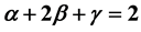combines the scaling laws resulting from the two relations and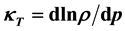. In the context with, the second temperature derivatives of the chemical potential and vapor pressure are investigated. As the critical point is approached, diverges as, while converges to a finite limit. This is explicitly pointed out for the two- phase fluid, water (with). The positive and almost vanishing internal energy of the one-phase fluid at temperatures above and close to the critical point causes conditions for large long-wavelength density fluctuations, which are observed as critical opalescence. For negative values of the internal energy, i.e. the two-phase fluid below the critical point, there are only microscopic density fluctuations. Similar critical phenomena occur when cooling a dilute gas to its Bose-Einstein condensate.

Keywords:

Critical Condition U = 0, Critical Opalescence, Rushbrooke Equation, Thermodynamic Fit Functions for Saturated Water, Vapor and Liquid Volumes, Vapor Pressure, Chemical Potential, Entropy, Internal Energy, Free Energy, Heat Capacity

1. Introduction

An essential property of matter is its structure, i.e. the distribution of its constituents in space and time as governed by inter-particle forces [1] . We are concerned here with the electrically and magnetically neutral single-component gas under steady-state conditions, which are thermodynamically defined in the immediate vicinity of the critical point and below it.

Andrews’s discovery of critical opalescence in carbon dioxide in 1869 stimulated numerous investigations of critical phenomena. The experimental observations on fluids show that a colorless gas in a narrow temperature range above its critical temperature suddenly becomes opaque and changes color and, at, exists as a two-phase fluid of different densities in volumes that are sharply separated by an interface surface a few molecular layers thick. The endeavor to explain theoretically the observations constituted a huge challenge. The course of a century then saw the development of the familiar phenomenological theories of a van der Waals gas, of the stable and unstable thermodynamic equilibrium formulated by Gibbs, of the correlation of fluctuations, of the scaling laws, including the hierarchical reference theory (renormalization group techniques), and of the Monte Carlo computer methods (see [2] ).

An insight into the nature of a fluid in the critical region is afforded by Figure 1, which for water of mass [g] and critical density in the volume [cm³] shows the different fluid states as a function of the temperature. Below, is distributed as condensed mass with the density in the sub-volume and as vapor mass with the density in the sub-volume. This gas in thermodynamic equilibrium existing in two phases is called a saturated fluid. As thermodynamic theory teaches, as the only independent variable of the saturated fluid that can be chosen is the saturation temperature, since the other field variables possible, viz. vapor pressure and chemical potential are unique functions of.

Every thermodynamic quantity of the saturated fluid, , can thus be represented as a function of. The absolute values both of the fluid, , and of the fluid phases, vapor, , and condensate (liquid, solid), , are proportional to the mass in the volume considered. As extensive quantities they have additive properties, i.e. they satisfy the equations

(1)

The mass-specific quantities and contain the complete thermodynamic information on the fluid state [3] . The difference gives the difference of the thermodynamic properties of in the volumes and and is called an order parameter. The quantity can be expressed by the quantities, , and:

(2)

The quotient is a function of the vapor pressure, and the quotient a function of the chemical potential:

(3)

and

(4)

The vapor pressure is a positive, convexly curved, monotonically increasing function of the temperature and the chemical potential a negative, concavely curved, monotonically decreasing function of the temperature. Open questions on the thermodynamic properties of and, in particular in the critical region, are dealt with in Sections 3 and 7.

Equation (2) can be transformed to

(5)

Equation (5) yield, for example,.

Relations (1)-(5) represent the Gibbs equations for calculating, , and of the saturated fluid. One might think that the job of setting up generally valid fit formulae, i.e. applicable to every two-phase fluid has already been done. But this is not so. The literature yields, e.g. for water, only formulae for industrial use ([4] - [6] ) which do not correctly give the physical picture of the two-phase fluid in the critical region.

The objective of this study is to represent the quantities, , and in the region between the triple point and the critical point as thermodynamic fit functions dependent on the temperature (Sections 4-9). The representation of a fit function by an order parameter expanded around the critical point is based on the knowledge of the behavior of the fluid in the critical region.

2. Thermodynamics of Critical Phenomena

The thermodynamical physics of critical phenomena above and below the critical point is extensively treated in the literature (e.g. [2] [7] -[10] ). Critical phenomena occur under the natural boundary condition of the vanishing value of the internal energy, [11] . In the immediate vicinity of the critical point the one-phase fluid is in unstable equilibrium on transition to the two-phase fluid, which is then in stable equilibrium.

Thermodynamics describes the macroscopic state of the fluid by means of the quantities, , , and and thus cannot delve into the microscopic processes actually occurring in the particle interactions taking place in the fluid. The effect of attractive and repulsive forces among interacting particles on the internal energy is that has negative sign for fluid temperatures below and positive sign above. can be treated as the sum of two energy contributions, viz. the potential energy, whose gradient yields the attractive forces, and the thermal energy, which is assigned to the sum of kinetic, vibrational and rotational particle energies. As the result, Figure 2 shows for saturated water (under the same conditions as in Figure 1) the internal energy and the estimates and in liquid and vapor as functions of the mean particle separation, represented by

the normalized density values in the regions with [K] and. For an estimation

it is taken for granted that the thermal particle energy increases proportionally as the saturation temperature,. The empirical value is given by [J/g]/273.16 [K] = 1.26918 [J/(gK)]. To calculate, is multiplied by the mass. This yields in the liquid phase an initially

expected increase and on reaching the maximum value 668 [J] at about, [K], [g] a continuous decrease to the critical value [J]. With the decrease is continued in the vapor phase. The product continuously decreases as the particle separation increases; at the value [J] is assumed. As

(with [g]) can be calculated according to Equation (5), it is possible to estimate the potential numerically. is always negative. The resulting repulsion and attraction forces between the particles are equal and opposite at the critical point, which is expressed in Figure 2 by the fact that the curves, , and all are continuous there. Qualitative information about mean-field strength of forces in liquid and vapor can be obtained from and.

The positive and negative regions of the fluid internal energy are shown in Figure 3 for water in the pressure vs volume diagram. They are separated by the isotherm above the critical pressure (dashed line) and the vapor pressure below and (solid line). Along the dashed line there is a continuous change in the density passing through positive and negative regions of. The solid lines represent the vapor pressure at temperature and are the loci of the first-order phase transition due to the jump between low-density vapor and high-density condensate. The jump is combined with a different fluid structure in each phase.

A fluid state of is characterized by an ensemble of particles freely moving in a structureless homogeneous phase. In contrast, a fluid state of is characterized by an ensemble of particles bound in a more or less structured form as a result of particle self-organization under certain constraints, e.g. liquid, solid, and Bose-Einstein condensate (BEC) [12] , each with its specific thermodynamic property. As an example, Figure 4 shows the variations in internal energy of vapor and condensates as functions of their phase-specific volumes and the saturation temperature, respectively, for the water mass of 1 [g].

The discontinuities of, represented as circles in Figure 5, indicate the phase transitions of bulks of different structures. States of different aggregation exhibit qualitatively different properties. Adding energy to the fluid at fixed temperature distributes a surplus of the one bulk phase at the expense of the other [1] . Local variations of internal energy couplings between particles change the bulk structures. A structural change is thermodynamically described by an increase in internal energy as a result of increasing system entropy, i.e. by. Changes in the bulk structure occur close to absolute zero, at the triple point and the critical point. The circles in Figure 1 and Figure 5 give the phase transitions for the functions, , , , , , and. It is seen that the phase transition near absolute zero at the critical temperature of the BEC, , refers to the mass, at to the mass, and at to the masses and, where it holds that. The discontinuous transition in the [K]

region from to is the consequence of the change from the condensed gas structure of the single quantum state of a BEC to the gaseous state of a collection of freely moving particles; this can only be treated with quantum mechanics (in a BEC experiment the energy is extracted from the mass). The continuous transition at fixed from to is thermodynamically treated as a phase transition of the first kind (the complete change from solid to liquid structures requires the energy that is called latent heat). The transition at from and to is thermodynamically treated as a phase transition of the second kind (the energy to be imparted to the masses and vanishes in the limit:, i.e. is not latent heat). The smooth and continuous regions aside the circles mark phase transitions between the homogeneous bulks, condensate and vapor. A transition at from the condensed phase to the vapor phase is likewise classed as a phase transition of the first kind (the vaporization enthalpy has to be provided).

It is of interest to explain the occurrence of macroscopic fluctuations under the conditions close to the critical temperature, , and their reduction to microscopic fluctuations under the conditions for. An unstable equilibrium position marks the beginning of decomposition of the mass to under the condition. On a macroscopic scale the binding potential of all particles, , restricts its averaged value to the averaged value at. The condition appears twice in the state diagram of a gas (Figure 5): both at high particle number and critical density cm in the vicinity of the critical point, , and also at low particle number of order and particle densities cm in the vicinity of the absolute zero,. The state, as in the case of critical opalescence, is macrocopically described by correlation functions, and the state, as in the case of a Bose-Einstein condensate, quantum mechanically by a

condensate wave function. As already mentioned, correlation functions are a measure of the number of scattering centres for light in the fluid dielectric and hence of a mean value of structural density fluctuations. The strong increase and subsequent decrease of long-wavelength fluctuations in critical fluid regions cause the observed sharp increase and decrease of scattered light intensity (e.g. [13] ) and are thus experimental proof of the thermodynamic zero of the internal energy of, on the one hand, a dense gas in the critical temperature region and, on the other, a dilute-gas in the K region.

Evidently, nature associates the problem of changing the sign of at with the ability of self- organization of particles interacting in ensembles. For, the statistically distributed thermal energy of free-moving particles, , outweighs the mutual binding energy, , yielding. With decreasing temperature, decreases and becomes more negative, as long as both terms cancel at

, i.e.. The deviation of the fluctuating energy variable from its average value is itself a fluctuating variable and the mean square deviation is a convenient measure of the magnitude of the fluctuations [3] . The energy fluctuations become enormously close to the critical point since is equal to. Together with density fluctuations, this represents an unstable equilibrium

of the fluid state. One of the best ways of finding solutions for realistic particle interactions under the condition is to compute the order-parameter probability distribution functions by means of Monte Carlo computer methods [10] . Computer simulations under different thermodynamic conditions afford quite a good picture of the phase transition in the critical region, and in conjunction with the renormalization group techniques allow calculation of critical exponents.

For the Gibbs applied theory, on the other hand, yields with Equations (1)-(5) universal order- parameter relations for calculating material-dependent critical exponents.

Van der Waals was the first to show that the normalized difference in the phase densities is empirically very well described by a power law of the form, in which the normalized temperature difference appears as a variable and the so-called critical exponent characterizes the decrease of as approaches (Figure 1). Applied thermodynamics has to determine the particular critical exponent for every order parameter, and, converging to zero. Here the value of the critical exponent depends on the choice of the variable of the order parameter. It is customary to choose the temperature as variable.

When thermodynamic relations between various thermodynamic functions are known, these will reappear in corresponding relations between their critical exponents. A well-known exponent equation for the saturated fluid (e.g. [7] ) is

(6)

(Rushbrooke equation), which describes the numerical relation between the exponents of the reciprocal heat capacity, the difference in the phase-specific volumes, and the reciprocal isothermal compressibility. The temperature dependences of these functions in the immediate vicinity of the critical point are defined by

(7)

Consequently, the task here is to repeat the calculation of and and additionally of the exponent of every function, which according to Relations (3) to (5) is connected with the heat capacity. Since

(8)

these are the functions, , , , , , , and. Obviously, is an important measurable quantity that yields information on the phase transition at. The knowledge obtained about the temperature dependence of the functions mentioned then allows relations between critical exponents to be studied, e.g. between, , and (Sections 4-9). It is found that only a single independent critical exponent is needed to characterize all order parameters, e.g. and the others can be expressed by it. Data for the fluid selected, saturated water, are given in the Appendix.

It remains to consider some essential properties of the above-mentioned free interface surface.

If the condition for forming a free surface between the liquid and vapor phases is given, then there is an interface particle layer, which represents a new equilibrium state described by a minimum internal energy and simultaneously a maximum entropy. Hence formation of the free interface surface lowers the free energy of the fluid. The relative energy contribution of an interface quantity to the respective system quantity depends on the ratio of the numbers of interacting particles in the interface volume (of the surface area

times the layer thickness) and system volume and is therefore extremely small. Despite the

smallness of the order and less, surface effects play a role in nature and technology, e.g. the minimization of the free interface surface. The smallness of an interface quantity shows, on the other hand, that ignoring it when studying volume properties of the fluid is completely justified. As the existence of a surface does not change the mass and volume, the property of, , and being extensive quantities is maintained.

If the area-specific difference of the internal energy is denoted by the temperature coefficient (surface energy), then the coefficient of the surface entropy increased at constant temperature, , is assigned to the function and that of the surface free energy decreased, , to, yielding the two-phase fluid-relations for:

(9)

Equations (9) give, , and as functions of the system variables, , and and their conjugate temperature variables, , and. In order to establish a relation between the unknown function and the measurable surface tension, it is posssible simply to identify the negative values with the free energy,

i.e.. It is found that this choice gives the acceptable result of interface- specific coefficients, viz., , and concave curvature, as shown in Figure 6 for water. The physical significance of

the negativity of and and the positivity of is readily apparent since these functions multiplied by represent area-contributions to the negative internal and free energies and positive entropy of the two-phase fluid.

3. Vapor Pressure

The experimental finding that the heat capacity diverges at the critical point calls for a statement on the critical behavior of the vapor pressure and chemical potential, since. What was known about the properties of these two quantities at the time when systematic investigations of the critical behavior of fluids and magnets were initiated [14] -[17] is summarized by Stanley [7] in his book (1971), Introduction to phase transitions and critical phenomena, as follows: If is divergent, then or or both will be divergent. The exponent is introduced as a measure of the degree of divergence (if any) of the curvature of the vapor pressure curve, i.e.. The lattice-gas model gives. However, for the real gas the curvatures of and might both indicate divergence, so that might differ from. In particular, the divergence of the heat capacity of helium-4 (He) appears to be dominated by

rather than by.

Since then investigators have become resigned to not making any statement on and letting grow as (e.g. [18] -[22] ). This attitude, however, is not accepted by all. In general, the literature provides no uniform statement on the temperature dependence of in the critical region. The findings range from the absence of divergence, e.g. in the case of helium-3, to explicit specification of the exponent, e.g. in the case of water [4] [5] .

We shall take up the problem and show that. If, on the other hand, the exponent is introduced in order to describe by the divergence of the curvature of the two-phase chemical potential, then is valid, as shown in Section 7.

In the one-phase critical region a distinction must be made between conditions at constant volume, pressure, and chemical potential since, , and. For example, the difference of the heat capacities is positive, , while it vanishes in the case of the two-phase fluid [11] . To describe phase transitions under various conditions at it is necessary to introduce some different independent critical exponents that are inter-related [10] [23] -[27] .

With respect to the vapor pressure, the necessary thermodynamic proof of the finiteness of in the critical region enlists the possibility of estimating the second temperature derivative by an expression containing as highest temperature derivative the first derivative, which itself is finite at the critical point. An estimate formula is obtained as follows. The vapor pressure can be expressed by the following relations:

, (10)

.

The function is defined by the ratio of the evaporation energy to the volume energy at the phase transition. This ratio, which is always greater than 1, decreases monotonically as the temperature rises because the binding energy difference, although its contribution to the heat of vaporization, , always exceeds that of the free energy difference, continuously decreases with rising temperature in proportion to. In other words, the function decreases with increasing:

Differentiating Equation (10) gives and . The term of interest here is . In the critical region the quotient has a well- defined value which does not essentially change in the limits and and can thus already be determined at a great distance from the critical point. It is finite and almost constant in the entire critical region.

From in the critical region it follows that and, because of for, the following etimate is generally valid:

(11)

The maximum value of is assumed at the critical point and is finite; it is thus shown that never diverges.

It will now be shown that no temperature derivative of the vapor pressure diverges at the critical point, where it holds that; this value can be calculated according to the scaling laws and and with is finite; the critical value is likewise finite. Since scales as, further differentiation of cannot generate a divergent term and always yields on the left-hand side a term with a derivative of one degree higher than on the right-hand side, which only contains terms whose values at the critical point are finite. Since, therefore, every derivative can be expressed by terms with which do not diverge at, does not diverge either. From this it follows that can be expanded about the critical point as a Taylor series.

Series expansion of

Since the derivatives exist for every integer and do not diverge, the temperature expansion of around is possible, yielding

. (12)

The -expansion (where and) reads

. (13)

The positive functions and increase monotonically as the temperature up to their finite critical values and, i.e. it holds that and for. The constants in the -expansion are found by fitting the given vapor pressure data.

A fit formula of conceptually different form, based on the expression (10) for the vapor pressure, is

, (14)

where and are reference values, e.g. the boiling temperature [K] at atmospheric pressure [MPa].

The usual representation of measured vapor pressure data in the form versus shows that

the data can be described in first approximation by the straight line through the boundary points and (see Figure 7). This linear function is

. (15)

If one introduces the dimensionless variable instead of the inverse temperature variable, is represented as a function of as follows:

(16)

The essential property of the function is that the derivatives exist

for arbitrary and remain finite for. This satisfies the above-stated thermodynamic requirements, viz. that may nowhere diverge in. Fine fitting with measured vapor pressure data calls for a further function, which, of course, is likewise arbitrarily often differentiable and nowhere diverges, and which together with as product function fits the values. As a function with fit constants, the finite power series

(17)

can perform the task required.

The first three derivatives of are, and. The -th derivative is.

If the -th derivatives of and are denoted for short by and, the -th derivative of is

(18)

With the binomial coefficients, i.e. the figures in the Pascal triangle, one can calculate all derivatives of the function and they are all finite in.

The following fit formula for the vapor pressure is conceived such, with due allowance for Equation (10), that it does not yield any divergent higher-order temperature derivative:

(19)

Each constant of the series (see Equation (17)) is multiplied by the prefactor

of (see Equation (16)), yielding the constant, which is again denoted by in the fit formula (19). Equation (19) can be used for describing the vapor pressure of every fluid. In the literature, however, one finds fit equations (e.g. in [4] [5] [22] ) that are thermodynamically incorrect, because the corresponding function contains terms with non-integer exponents (e.g. terms such as or) that lead to divergences of

for.

Formula (19) with the ten fit constants listed in the Appendix, Equation (A3), reproduces the measured data of water with the same accuracy as that given in [4] -[6] . The calculations of in this study and, on the other hand, according to the equations published in [4] and [5] show that the differences expected occur exactly in the critical region, as seen in Figure 7. Results of calculating the water vapor pressure according to Equations (13), (14), and (19) are given in the Appendix (fit functions (1)-(3)).

4. Coexistence Curve

Along the coexistence curve in the critical region, the scaling laws must of course obey each two-phase equilibrium relation, e.g., and at the critical temperature the limits [11] :

(20)

In accordance with the defining Equation (7) for the exponent one obtains the scaling laws of the phase- specific volumes, internal energies and entropies in relation to their critical values as follows:

(21)

In these formulae the plus sign refers to the vapor phase and the minus sign to the liquid phase. According to van der Waals the temperature dependences of the volumes and can be represented as series expansions about the critical value, where the temperature expansion variable gives the distance to the critical point and at the same time the decrease of the difference, which both tend to zero on approaching the critical point:

(22)

The expansion variable is then expressed by the power function

(23)

The temperature dependence of is described by, is a positive constant, and is the

exponent defined by the function under consideration, for example, for the functions. The definition range for and restricts the range of values of and. For

saturated fluids one has and can assume a positive or negative value. The smaller a positive exponent is, the deeper the approach of the function to zero. A negative corresponds to a function which diverges to infinity at the critical point. An exponent leads to a series expansion with no anomalous behavior as, for example, the vapor-pressure difference in Equation (13). The properties stated are also exhibited according to Equation (21) by the functions and, where.

5. Critical Exponents of the Phase-Specific Quantities and

According to Equation (3) a quotient has a finite value at every temperature. It thus follows that

(24)

According to Landau every quantity between the stable phase-limiting values and, whose difference, as described in Equation (24), tends to zero on approaching the critical state, is based on an order parameter [28] . In the case of the saturated fluid the natural order parameter is the difference of the

condensation and vapor masses in relation to the fluid mass,. The ratios and can be expressed by the quotients and. If the value in is expressed by, which is justified in the critical region (see curves 1 and [1] in Figure 8), then is identical to.

The variable thus represents the order parameter of the mass splitting, which as natural order parameter of the two-phase fluid is also the basis of all other order parameters:

(25)

For values, the phase-specific volumes and internal energies on the coexistence curve conform to the scaling functions,

(26)

The values of and can be determined empirically by varying them until the curves of the published data (curves 2 and 3) and the scaling laws (straight lines [2] [3] ) satisfactorily converge in the critical region as shown

for water in Figure 8. From Figure 9 it is seen that relations (26) are valid for and hence for. One obtains, , ,. With one gets, , , , , , , , , .

It can now be stated that the phase-specific quantities and in relation to their critical value scale as:

(27)

In contrast, the temperature derivatives scale as; they diverge at the critical point where because:

(28)

Calculation of and yields with

(29)

The relation, claimed by Ref. [11] , is wrong and must be replaced by Equation (29). The divergence also follows from

and

.

To get temperature-dependent quantities in the entire temperature range of the liquid, the given data and are fitted and represented as power series. Here is chosen as

independent variable with values between 0 and 1, and is replaced by. A fit function expanded about the critical point with the exponent is then

(30)

The sum contains constants which are specific to the quantity to be fitted and are calculated by the mathematical method of conjugate gradients by fitting the given data. Quantities such as the vapor functions

, , , , , and the corresponding liquid functions as well as the differences are expressed in terms of the fit function (30). It is found that constants is

sufficient to generate data with the numerical exactness usual in the literature. Results are stated in the Appendix, see fit functions (5)-(26).

6. Critical Exponent of the Fluid Energy

First it is shown that the internal energy is an order parameter:

At one has and [11] , i.e..

Each of the following functions has the property of an order parameter since it holds that, , , , and.

To obtain the fluid quantity as a function of, Relation (2) is transformed as follows:

(31)

The fluid quantity in relation to its critical value (which takes either the minimum or maximum of) scales as:

(32)

In the case one obtains with

(33)

Below, is a negative function which tends to zero in the critical region as or. The temperature derivative is a positive function and scales as:

(34)

For, diverges as.

Quantities such as the fluid functions, , , , and are fitted by the fit function

(35)

See Appendix, fit functions (27)-(33). In particular, from one has, because of and [16] , the scaling.

7. Critical Exponents of the Heat Capacity and Chemical Potential Functions

The scaling of, taking Relations (4) and (26) into account, is calculated as follows:

(36)

Thus, tends to the final value, while the difference converges to zero as:

(37)

This agrees with Equation (5). Differentiation of yields

(38)

The scalings of and are with described by Equation (34) and the scaling of is calculated from the difference:

(39)

The (positive) functions and diverge for as, while the (negative) function converges as to 0. The exponent of is denoted in accordance with Equation (7) by; is thus holds that. The identity

(40)

thus states that the heat capacity function is the temperature derivative of the internal energy function, whose exponent is. From the scaling it follows that the function converges to zero as and the function as, where are constants. See Appendix, fit functions (38) and (39).

8. Critical Exponent of the Reciprocal Isothermal Compressibility of the Two-Phase Fluid

The isothermal compressibility is measured as the relative change of the fluid volume when the pressure is increased, i.e. the reciprocal isothermal compressibility is defined by the relations:

(41)

In the one-phase region the density and pressure increase monotonically along an isotherm and one gets the relations with the value at the critical point [14] . In the two-phase region, on the other hand, the vapor pressure and densities remain constant at constant temperature, and one has to consider how a mechanical quantity such as the isothermal compressibility is to be interpreted here. Any attempt to compress the fluid of constant density is accompanied by condensation of the vapor mass and release of energy, which results in a temperature increase by, this in turn leading to the pressure increase. The isothermal compressibility is therefore infinite except on the coexistence boundary when the fluid becomes homogeneous on the liquid side. Representation of the connection between vapor pressure and phase densities along the coexistence curve allows the difference to be introduced as a density function, whose pressure dependence is a well-defined negative quantity with the reciprocal value at the critical point.

Justification for choosing and can be given by treating the isothermal compressibility according to the Le Chtelier-Braun princple [3] . The change of state is described as the two infinitesimal changes of states, viz. and, which process simultaneously and are indirectly induced since. The change of state, , is an isothermal variation of the entropy and volume, , which according to Equation (3) is expressed by the isothermal phase transition. The isobaric volume compression, , is expressed by. The change is the result of the temperature increase or the vapor pressure increase since. Hence the effect of the isothermal and isobaric infinitesimal changes on the two-phase fluid of constant density is

(42)

Calculating the scaling of gives

(43)

and yields the exponent of the two-phase fluid:

(44)

The function is represented in Figure 10 for the case of water; in the

critical temperature region it goes asymptotically to zero with the proportionality factor. Measurements of under one-phase conditions for water liquid and gas about the critical region are performed by Ref. [29] , yielding.

9. Fit Functions for the Saturated Fluid

To describe important thermodynamic properties of the saturated fluid, fit functions of quantities are set up. A fit function presents an appropriate power series expanded about the critical point and affords the possibility of obtaining fairly reliable information concerning the thermodynamic function. Of course, the exponent of the series is defined by the thermodynamic function. Calculation of the fit constants is done by the least squares method, published and estimated data taken as a basis. Fit functions are evaluated for water data (see Appendix). The tables each (arbitrarily) list 10 fit constants, with the aid of which each temperature value of the

thermodynamic quantity in the region can then be calculated. As an example, some evaluated functions are represented in Figure 11, viz., , , , , and.

10. Results and Discussion

The Gibbs theory describes the macroscopic state of matter by means of the quantities, , , and

and thus cannot delve into the microscopic processes of interacting particles which give the structure of matter. Nevertheless, the theory treats the thermodynamic equilibrium of matter correctly, using interrelations between the entropy, internal energy, chemical potential, pressure, and temperature. If an additional parameter, , is introduced for characterizing the behavior of any thermodynamic quantity under the boundary condition of a reversible isobaric and isothermal transition from the condensate structure to vapor, it follows that this reveals in all thermodynamic relations relevant to these changes. For the two-phase fluid, the established Gibbs interrelations are summarized by Equations (1)-(5). Equations (8) explicitly show relations between the heat capacity, free energy, entropy, internal energy, vapor pressure plus chemical potential, and phase-specific heats and volumes as functions of the temperature and, consequently, the parameter. Then a specific quantity is formulated, according to van der Waals, in terms of a power series expanded about the critical point as a function of and, which is called a thermodynamic fit function. It is valid between the critical and triple points. Thermodynamic fit functions for 40 two-phases quantities are listed in the Appendix. They are given as functions of the temperature variable and characterized by fit parameter arrays and. The figures proposed here are specified for saturated water.

The critical point is thermodynamically defined by the vanishing value of the internal energy, and this and Nernst’s allow calculation of all thermodynamic functions with absolute figures and the unique transformation of one plotted projection plane into another.

Regarding the scaling on approach to the critical point, it is found that the phase-specific volumes, entropies, and energies are dominated by the critical exponent, and the fluid entropy and energy by, while the second temperature derivative of the chemical potential by, thus determining the divergence of the heat capacity. The second temperature derivative of the vapor pressure converges to a finite value. The difference of phase-specific quantities likewise scales as and the sum scales as.

The exponents of the reciprocal heat capacity, , and reciprocal isothermal compressibility, , calculated for the two-phase fluid are not in conformity with those given in the literature for the one-phase fluid. The corresponding exponents differ since the thermodynamic behavior above and below is described by different free energy functions [14] . There are large density fluctuations in the immediate vicinity of the critical point under the condition. These unstable fluctuations do not occur under the condition and are not the subject of the Gibbs theory, which deduces the thermodynamic stable equilibrium of the macroscopic fluid from the statistics of microscopic fluctuations of its constituents at given total energy.

The subject of quantum mechanics is to investigate in detail interactions between particles. There are statistical arguments about the relative likelihood of attractive and repulsive interactions. In particular, one has to consider the possible resonant scattering of particles with different internal degrees of freedom and spin- exchange and dipolar processes [12] . This is all very hard to do, but it may finally provide an explanation for large density and energy fluctuations in a fluid in the vicinity of. On the other hand, atto- and femtosecond laser techniques have made it possible to follow the movements of atoms and study subpicosecond processes in solids and liquids as well as in gases (in and out of the direct light interaction region) [31] .

Almost all significant results produced in the years 1960-1980 were obtained at a time when non-classical thermodynamic behavior of the free energy of the one-phase fluid near the critical point is assumed. The efforts to obtain an equation of state that describes the singularities of the heat capacity and isothermal compressibility in the critical region are to be found in, for example, Refs. [14] -[16] , and [29] . As is shown in this study, however, the scaling laws of the two-phase fluid can be treated on the basis of the classical thermodynamic free energy function if the equilibrium relations between the phase-specific volumes, vapor pressure, chemical potential, and heat capacity are considered. A significant result is thus confirmation of the Rushbrooke equation for the two-phase fluid. It is satisfied by the van der Waals gas because, , and, and for the real two-phase gas because and, with having a value smaller than. Since the exponent of the internal energy is, the Rushbrooke equation can be interpreted as the sum of the exponents of the reciprocal heat capacity, internal energy, and reciprocal isothermal compressibility.

The appreciable deviations of the two-phase fluid values calculated here, and (in case of saturated water,), in relation to those given for the real one-phase fluid in the literature, e.g. Ref. [23] , , , and, are very surprising indeed. Such eminently different results can be explained, as mentioned above, by the statements that the scaling hypothesis, in particular the renormalization group techniques, is valid for one-phase fluids where and, but is not suitable to represent the behavior of two-phase fluids where and [11] .

Nature reveals the thermodynamic energy zero of a gas at the critical point through the sudden appearance of macroscopic fluctuations in a narrow temperature range above. The critical behavior depends on particle interactions, thus the equilibrium conditions of fluid stability and instability and the size of fluctuations in the vicinity of have to be regarded. The condition means that the positive internal energy contribution of the thermal energy of all fluid particles, , balances the negative internal energy contribution of the binding energy of all particles,. Under the condition the inter- particle forces of attraction and repulsion cancel. This leads to an unstable equilibrium of one-phase particles and hence local density fluctuations, , of wavelengths of order Å [1] . If, however, the mass in is split up into the condensed mass of overbalanced bound particles with and into the vapor mass of overbalanced freely moving particles with, then there is no eventuality of macroscopic fluctuations, i.e. the masses and are in stable equilibrium within the subvolumes and, respectively. Conditions for macroscopic fluctuations and hence observation of critical opalescence exist near to the critical point where particles, , and

, and close to absolute zero where particles, , and (gaseous state). In the BEC state where macroscopic density fluctuations are suppressed and alone microscopic fluctuations occur, yields the condition precedent for the existence of coherent matter waves.

Changes in the fluid structure take place at phase transitions where the gradient is not

continuous in the representation (Figure 5). This is the case at the critical point of the Bose- Einstein condensate when the BEC changes to the dilute gas, at the triple point when the solid continuously melts to liquid, and at the critical point of the fluid when the two phases disappear. The first two phase transitions mentioned are associated with heat input required to alter the fluid structure and are called phase transitions of the first kind, whereas the phase transition at the critical point occurs without additional energy and is called a phase transition of the second kind. Every isothermal transition at from the condensate to the vapor state, which requires the energy input, is a phase transition of the first kind.

Adding energy to the fluid increases its entropy and thus the mobility of particles, both being equivalent to a loss of matter structure. This feature can be described by the concept of an order parameter. The “natural” order

parameter of the two-phase fluid is (Equation (25)), but specific order parameters may be used to specify fit functions, e.g., , and, to describe entropic, energetic or volumetric first-kind phase transitions (see Appendix).

Area-specific order parameters are the surface energy and surface tension. They describe the effect of particle interactions in the highly inhomogeneous interface layer at the free area between the homogeneous bulks, condensate and vapor. Since is part of the fluid internal energy, which is negative below the critical point, must be negative and the temperature values can be determined according to Equation (9), if

is set equal to the negative temperature values of. As part of the fluid free energy, lowers the free system energy when the fluid proceeds to a new equilibrium state with an interface layer. Interesting enough, the zeros of the surface energy and surface tension, viz. and at on approaching the critical point from below, evidently display the disappearance of the free interface surface and through the occurrence of the thermodynamic internal energy zero of the high-density fluid, since.

The thermodynamic internal energy zero of the low-density fluid is the vanishing value at the critical temperature of the BEC, i.e.. The internal gas energy is positive above and negative below, when all gas particles suddenly condense into a quantum state (Figure 5, where). The lowest energy is assumed by the quantum state of zero momentum, zero entropy and zero temperature [3] .

Acknowledgements

The author would like to thank the Max Planck Institute of Plasma Physics (IPP), Garching, for providing computing facilities. He is also grateful to K. Dodds-Eden, D. Düchs, S. Wipf, and H. P. Zehrfeld for helpful discussions and to A. M. Nicol for the English translation.

Cite this paper

AlbrechtElsner, (2014) Thermodynamic Fit Functions of the Two-Phase Fluid and Critical Exponents. Engineering,06,789-826. doi: 10.4236/eng.2014.612076

References

Appendix: Fit Functions for Thermodynamic Properties of a Saturated Fluid in Liquid-Vapor Equilibrium

Computer program for evaluating fit functions

Temperature values of a specific thermodynamic quantity are calculated by calling the IDL-FUNCTION evaluation in an IDL-source program:

The IDL-FUNCTION evaluation is specified by the label, e.g., that is relevant to the selected fit function, the fit arrays and, and the temperature variable of. The general structure of an IDL evaluation function is given below.

In this work the following values are fixed, valid for saturated water:

In addition, the values

are specific for calculating an individual thermodynamic fluid quantity. These are listed by. A thermodynamic quantity is thus described by, , and as a function of the temperature variable, where for instance・findgen (1234)/(12341).

FUNCTION evaluation, k, a, b, x

The fit function with label=1 evaluates the vapor pressure Equation (13)

(A1)

The fit function with label = 2 evaluates the vapor pressure Equation (14)

(A2)

The fit function with label = 3 evaluates the vapor pressure Equation (19)

(A3)

Fit functions for saturated water

Each of the fit functions, , yields the vapor pressure

(1-3) vapor pressure [J/cm³]

Fit function yields the reciprocal isothermal compressibility

(4) reciprocal isothermal compressibility [J/cm³]

Fit function yields for quantities (5)-(26).

According to Equation (30), this function calculates functions with exponents.

(A4)

(5) order parameter

(6) relative liquid mass

(7) liquid volume [cm/g]

(8) vapor volume [cm/g]

(9) vapor volume-pressure energy [J/g]

(10) liquid volume-pressure energy [J/g]

(11) specific free energies difference [J/g]

(12) specific entropies difference [J/(gK)]

(13) specific enthalpies difference [J/g]

(14) specific internal energies difference [J/g]

(15) specific heats difference [J/(gK)]

(16) vapor density [g/cm]

(17) liquid density [g/cm]

(18) densities difference [g/cm]

(19) vapor internal energy [J/g]

(20) liquid internal energy [J/g]

(21) vapor enthalpy [J/g]

(22) liquid enthalpy [J/g]

(23) vapor entropy [J/(gK)]

(24) liquid entropy [J/(gK)]

(25) vapor free energy [J/g]

(26) liquid free energy [J/g]

Fit function yields for quantities (27)-(33). According to Equation (35), this function calculates functions with lowest exponent.

(A5)

(27) densities sum [g/cm]

(28) specific internal energies sum [J/g]

(29) specific entropies sum [J/(gK)]

(30) entropy [J/(gK)]

(31) internal energy [J/g]

(32) free energy [J/g]

(33) chemical potential function [J/g]

Fit function yields for quantities (34)-(35). According to Equation (28), this function calculates functions with lowest exponent.

(A6)

Fit function yields for quantities (36)-(37). According to Equation (38), this function calculates functions with lowest exponent.

(A7)

(34) specific heat of vapor [J/(gK)]

(35) specific heat of liquid [J/(gK)]

(36) heat capacity [J/(gK)]

(37) chemical potential function [J/(gK)]

Fit function yields for the quantity (38). This function calculates the temperature derivative of the chemical potential

(A8)

(38) chemical potential function [J/(gK)]

Fit function yields for the quantity (39). This function calculates the chemical potential

(A9)

(39) chemical potential function [J/g]

Fit function yields for the quantity (40). This function calculates the surface tension

(A10)

(40) surface tension [dyne/cm] or [erg/cm]

References

- 1. Stierstadt, K. (1989) Physik der Materie. VCH Verlag, Weilheim, Chapters 3.4, 10.2, 21.1
- 2. Domb, C. (1996) The Critical Point. Taylor & Francis Ltd, London, Chapters 1, 2, 6.2.4
- 3. Callen, H.B. (1960) Thermodynamics. John Wiley & Sons, Chapters 8.1-8.3, 10.4, 15, Equation (7.35).
- 4. Grigull, U. and Schmidt, E. (1989) Properties of Water and Steam in SI Units. Springer-Verlag, Berlin, T,s-Diagram, p. 205, Equation 1.
- 5. Wagner, W. and Pruss, A. (1993) International Equations for the Saturation Properties of Ordinary Water Substance. Revised According to the International Temperature Scale of 1990. Journal of Physical and Chemical Reference Data, 22, 783-787. The IAPWS Formulation 1995 for the Thermodynamic Properties of Ordinary Water Substance for General and Scientific Use. Journal of Physical and Chemical Reference Data, 31 (2002), 387-535.
http://dx.doi.org/10.1063/1.555926 - 6. Kohlrausch, F. (1996) Praktische Physik. Band 3, Teubner Verlag Stuttgart, Tabelle 3.12.
- 7. Stanley, H.E. (1971) Introduction to Phase Transitions and Critical Phenomena. Clarendon Press, Oxford, Chapters 1.1.1, 3.1, 3.4.2, 7.2.
- 8. Liu, Y. and Suzuki, M. (1987) Some New Developments of the Scaling Theory of Transitient Phenomena. Phase Transitions, 10, 303-314.
http://dx.doi.org/10.1080/01411598708215447 - 9. Kadanoff, L.P. (2009) More Is the Same; Phase Transitions and Mean Field Theories. Journal of Statistical Physics, 137, 777-797.
http://dx.doi.org/10.1007/s10955-009-9814-1 - 10. Plascak, J.A. and Martins, P.H.L. (2013) Probability Distribution Function of the Order Parameter: Mixing Fields and Universality. Computer Physics Communications, 184, 259-269
http://dx.doi.org/10.1016/j.cpc.2012.09.014 - 11. Elsner, A. (2012) Applied Thermodynamics of the Real Gas with Respect to the Thermodynamic Zeros of the Entropy and Internal Energy. Physica B: Condensed Matter, 407, 1055-1067.
http://dx.doi.org/10.1016/j.physb.2011.12.118 - 12. Pethick, C.J. and Smith, H. (2004) Bose-Einstein Condensation in Dilute Gases. Cambridge University Press, Cambridge, Chapter 5, Cover Illustration.
- 13. White, J.A. and Maccabee, B.S. (1971) Temperature Dependence of Critical Opalescence in Carbon Dioxide. Physical Review Letters, 26, 1468-1471.
http://dx.doi.org/10.1103/PhysRevLett.26.1468 - 14. Widom, B. (1965) Equation of State in the Neighborhood of the Critical Point. Journal of Chemical Physics, 43, 3898-3905
http://dx.doi.org/10.1063/1.1696618 - 15. Fisher, M.E. (1967) The Theory of Equilibrium Critical Phenomena. Reports on Progress in Physics, 30, 615-730.
http://dx.doi.org/10.1088/0034-4885/30/2/306 - 16. Rehr, J.J. and Mermin, N.D. (1973) Revised Scaling Equation of State at the Liquid-Vapor Critical Point. Physical Review A, 8, 472, Equations 2.8 and 5.5.
- 17. Heller, P. (1967) Experimental Investigations of Critical Phenomena. Reports on Progress in Physics, 30, 731-826.
http://dx.doi.org/10.1088/0034-4885/30/2/307 - 18. Wagner, W. (1973) New Vapour Pressure Measurements for Argon and Nitrogen and a New Method for Establishing Rational Vapour Pressure Equations. Cryogenics, 13, 470-482.
http://dx.doi.org/10.1016/0011-2275(73)90003-9 - 19. Stewart, R.B. and Jacobsen, R.T. (1989) Thermodynamic Properties of Argon. Journal of Physical and Chemical Reference Data, 18.
- 20. Gilgen, R., Kleinrahm, R. and Wagner, W. (1994) Measurement and Correlation of the (Pressure, Density, Temperature) Relation of Argon, II. Saturated-Liquid and Saturated-Vapour Densities and Vapour Pressures Along the Entire Coexistence Curve. Journal of Chemical Thermodynamics, 26, 399-413.
http://dx.doi.org/10.1006/jcht.1994.1049 - 21. Tegeler, Ch., Span, R. and Wagner, W. (1999) A New Equation of State for Argon Covering the Fluid Region for Temperatures from the Melting Line to 700 K at Pressures up to 1000 MPa. Journal of Physical and Chemical Reference Data, 28, 779-850.
http://dx.doi.org/10.1063/1.556037 - 22. Span, R. and Wagner, W. (1996) A New Equation of State for Carbon Dioxide Covering the Fluid Region from the Triple Point Temperature to 1100 K at Pressures up to 800 MPa. Journal of Physical and Chemical Reference Data, 25, 1509-1596.
http://dx.doi.org/10.1063/1.555991 - 23. Parola, A. and Reatto, L. (1995) Liquid State Theories and Critical Phenomena. Advances in Physics, 44, 211-298, Table 1, Chapter 5.5, Figure 15.
- 24. Zhong, F. and Meyer, H. (1995) Density Equilibration near the Liquid-Vapor Critical Point of a Pure Fluid: Single Phase T > Tc. Physical Review E, 51, 3223-3241.
http://dx.doi.org/10.1103/PhysRevE.51.3223 - 25. Rowlinson, J.S. (1959) Liquids and Liquid Mixtures. Butterworths Scientific Publications, London, Chapter 3.4.
- 26. Mouritsen, O.G. (1984) Computer Studies on Phase Transitions and Critical Phenomena. Springer-Verlag, Amsterdam.
http://dx.doi.org/10.1007/978-3-642-69709-8 - 27. Potton, J.A. and Lanchester, P.C. (1985) Analysis of Critical Specific Heat Data. Phase Transitions, 6, 43-57.
http://dx.doi.org/10.1080/01411598508219890 - 28. Landau, L.D. and Lifshitz, E.M. (1980) Statistical Physics. Part 1, Pergamon Press, Oxford, 449.
- 29. Levelt Sengers, J.M.H. and Greer, S.C. (1972) Thermodynamic Anomalies near the Critical Point of Steam. International Journal of Heat and Mass Transfer, 15, 1865-1886, Figure 4.
- 30. Schomacker, H. (1973) Messungen der inneren Energie und der spezifischen isochoren Warmekapazitat in der Umgebung des kritischen Zustands von Wasser. Thesis Ruhr-Universitat Bochum, Tabelle 1 und 2.
- 31. Milonni, P.W. and Eberly, J.H. (2010) Laser Physics. Wiley & Sons, Hoboken, Chapter 16.
http://dx.doi.org/10.1002/9780470409718