Engineering
Vol.6 No.6(2014), Article ID:46262,14 pages DOI:10.4236/eng.2014.66034
Peridynamic Solutions for Timoshenko Beams
E. Thomas Moyer, Michael J. Miraglia
Naval Surface Warfare Center/Carderock Division, W. Bethesda, USA
Email: Erwin.Moyer@navy.mil
Copyright © 2014 by authors and Scientific Research Publishing Inc.
This work is licensed under the Creative Commons Attribution International License (CC BY).
http://creativecommons.org/licenses/by/4.0/


Received 4 February 2014; revised 4 March 2014; accepted 11 March 2014
ABSTRACT
Peridynamics is a recently developed formulation for continuum mechanics which describes material deformation using a nonlocal approach. Unlike Classical Continuum Mechanics (CCM) where the conservation equations are cast into partial differential equations, Peridynamics describes the deformation in terms of integro-differential equations. Additionally, peridynamics permits a natural length scale that is absent in CCM. This facilitates the modeling of complex material behavior and fracture which is not dependent on the numerical discretization length scale. In this paper, we develop a Peridynamic formulation for a Timoshenko beam. Full details and numerical examples are presented for both bending and axial behavior. While the development in this paper is limited to elastic, infinitesimal deformations, the approach can be extended to finite inelastic deformations.
Keywords:Peridynamics, Timoshenko Beam, Beam Bending, Dynamic Deformation

1. Introduction
Peridynamics was introduced in 2000 [1] as a non-local theory for modeling the deformation of solid materials subjected to mechanical loading. The approach is well suited for dealing with problems containing cracks and discontinuities including the modeling of non-colinear crack growth [2] [3] . The formulation does not require spatial derivatives, naturally modeling discontinuous phenomena where fields are integrable but not differentiable [4] (e.g. cracks and discontinuities). A vast body of literature has been developed for various problems which include composite mechanics (e.g. [5] ), thermo-mechanical problems (e.g. [6] ) and various theoretical papers (e.g. [7] [8] ). A complete bibliography of the peridynamic literature is beyond the scope of this work; however, recent doctoral dissertations (e.g. [5] [9] ) provide a more comprehensive review of the literature.
The majority of the work to date has focused on solid mechanics applications where the equations of motion are developed for translational deformation in 1, 2 or 3 translational degrees of freedom (DOF). There has been little work to date investigating peridynamic formulations for structural mechanics (beams, plates and shells) where rotational DOFs are considered. This paper provides a complete solution for the deformation of a microelastic peridynamic Timoshenko beam. The formulation follows the traditional Timoshenko beam theory by considering extensional deformation, bending deformation and torsional deformation independently. Peridynamic deformations, analogous to traditional beam theory, can be obtained from the superposition of these three deformation modes. The problem is formulated for micro-elastic materials undergoing infinitesimal deformations. Work is in progress to extend the theory for finite deformations as well as inelastic material behavior.
Section 2 of this paper summarizes the theoretical formulation of an elastic rod which was introduced in the seminal paper on peridynamics by Dr. Silling in 2000 [1] . A numerical solution considering Dirichlet boundary conditions is presented and an example verification problem is solved. The static peridynamic solution reduces to the static continuum solution independent of horizon and grid spacing (assuming numerical convergence for all cases). Similar 1-D numerical solutions are explored in [10] . Section 3 presents a derivation for the bending of a Timoshenko beam including transverse shear effects. As is traditional for peridynamic formulations, it is derived from an assumed micro-potential leading to the peridynamic forces. An example problem with Dirichlet boundary conditions is solved and compared with the reference solution. Section 4 considers the more typical problem with mixed Dirichlet and Neumann boundary conditions. An example problem with reference analytical solution is solved. While not explicitly shown, the approach for mixed boundary condition axial deformation problems is identical to the approach for bending. Section 5 provides a discussion on the general solution for full 3-D deformation of Timoshenko beams followed by Section 6 with conclusions.
2. Peridynamic Elastic Rod—Numerical Solution
The discrete equation of motion for the infinitesimal deformations in a micro-elastic peridynamic rod with viscous damping is written as:
 (1)
(1)
where  represents the deformation at a point xi in the domain of the problem, A is the cross-sectional area of the rod, c is termed the micro-elastic constant, ρ is the mass density, cd is the damping constant and b(xi, t) is the body force. The integral is evaluated over a finite length of the rod termed the horizon. The distance, ε, is measured from the reference point to the integrand point as shown in Figure 1.
The rod is discretized with a uniform grid spacing of Δ, then  and the spacing is Δ = L/(n‒1) where L is the length of the rod. The choice of horizon is independent of the grid spacing but will be restricted for numerical convenience to be δ = mΔ. If we divide (1) through by ρ, assume the absence of body forces and restrict ourselves to Dirichlet boundary conditions we can write:
 (2)
(2)
where:
 (3)
(3)
The Dirichlet boundary conditions are given in the form:
 (4)
(4)
If we designate:
 (5)
(5)
We obtain the following system of 2nd order ODEs to solve numerically:
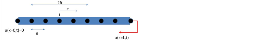
Figure 1. Schematic for 1-D rod peridynamic formulation.
 (6)
(6)
We choose to temporally integrate (6) using the Leapfrog Velocity Verlet scheme [11] with fixed time step, dt, which yields:
 (7)
(7)
 (8)
(8)
 (9)
(9)
 (10)
(10)
 (11)
(11)
For the purposes of the examples in this section, we assume homogeneous initial conditions so that:
 (12)
(12)
The peridynamic integral is evaluated using composite trapezoidal rule. It is most convenient to write Ii as the sum of three integrals:
 (13)
(13)
Starting with the 2nd integral term, which is included for any choice of the horizon, we obtain:
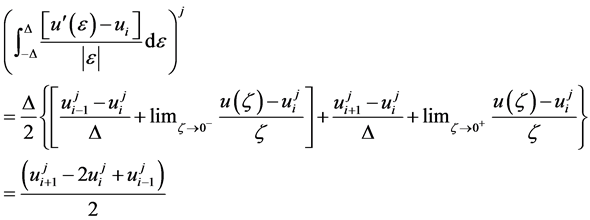 (14)
(14)
The first integral can be cast into the sum:
 (15)
(15)
where
 (16)
(16)
Similarly, the third integral can be cast into the sum:
 (17)
(17)
 (18)
(18)
Combining, we can compute  as:
as:
 (19)
(19)
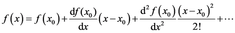
Examining the peridynamic integral for horizons which extend beyond nearest neighbors, it is evident the horizon extends outside the physical domain as one approaches the ends of the rod. If one simply assumes the micro-elastic modulus drops to zero outside of the physical domain (which is a perfectly valid peridynamic assumption), the material within 1/2 the horizon length of either end are “artificially” too hard or too soft (depending on the boundary condition) when comparing to Classical Continuum Mechanics (CCM). This is not surprising since truncating the micro-elastic modulus introduces a mathematical discontinuity which is inconsistent with the requirement in the CCM for u(x) and  to be continuous in the physical domain. To recover a solution which reproduces the results of CCM, one can consider a virtual extension of the physical domain which extends 1/2 horizon length beyond each physical end. The solution at any point outside of the physical domain can be approximated assuming a 1 term Taylor series expansion into the virtual material. So, for the case of points x < 0 and x > L we obtain:
 (20)
(20)
 (21)
(21)
The algorithm presented above provides a formulation which yields a peridynamic solution which approximates CCM in the static limit (assuming Dirichlet boundary conditions). For problems with time dependent Dirichlet boundary conditions the well documented dispersive characteristics of the peridynamic solution will be evident [2] [3] . These aspects will be demonstrated with a simple example below.
Example 1: Micro-Elastic Rod with Transient Sinusoidal Loading Consider the special case of a steel rod with the following parameters:
E = 3.0 + 7 psi
ρ = 7.324e-04 Pound-s2/in4 L = 100 inches The rod is fixed at x = 0 and the following boundary condition is applied at x = L
 (22)
(22)
This provides a transient response which settles down to the steady state when damping is employed. For this example, we employed 10% critical damping at the first harmonic of the rod. The driving frequency, fd, is three times the first harmonic.
Figure 2 shows the transient response at the center of the rod for the full time analyzed.
As expected, the response damps to the static solution independent of horizon length (equivalent to the CCM static solution). The value, δ, refers to the horizon which spans −δ <=> δ, δ = dx corresponds to nearest neighbor horizon where δ = 10dx corresponds to a horizon spanning 10dx (where dx is the grid spacing). The physical dimension of δ is 1 inch in this example and the grid spacing is adjusted accordingly. Figure 3 shows an enlarged section of the early transient response.
The well-known variable dispersion characteristics of the horizon [2] are demonstrated. With a nearest neighbor horizon, the peridynamic solution is equivalent to a finite difference solution of CCM. With δ = 10dx, the dispersion produces high frequency content during the transient response with diminishing amplitude due to the damping.
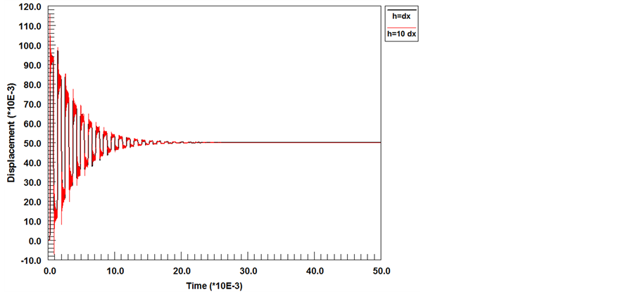
Figure 2. Center displacement for transient response of end driven rod.
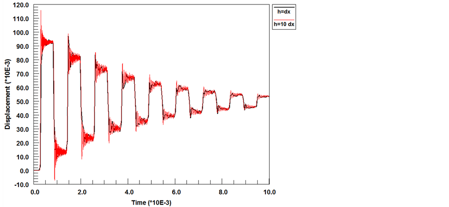
Figure 3. Early time center displacement showing dispersive behavior of peridynamic solution.
The well-known variable dispersion characteristics of the horizon [2] are demonstrated. With a nearest neighbor horizon, the peridynamic solution is equivalent to a finite difference solution of CCM. With δ = 10dx, the dispersion produces high frequency content during the transient response with diminishing amplitude due to the damping.
3. Peridynamic Formulation for Micro-Elastic Timoshenko Beam
Consider the bending deformation for a straight beam using the Peridynamic approach (Figure 4). The equilibrium equations for transverse force and bending moment are written as shown in (23) and (24) respectively.
 (23)
(23)
 (24)
(24)
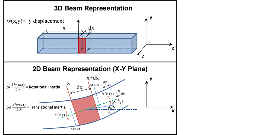
Figure 4. Bending Behavior Of A Timoshenko Beam.
where  is a reference point with a bound to a point given by
 , and:


For analogy to the Timoshenko beam theory, the shear force density at a point for a linear micro-elastic material takes the form:
 (25)
(25)
The rotational inertia induced in Timoshenko Beam Theory is due to two sources: rotational effects due to pure shear in the cross-section and the bending moment induced by the differential change in normal rotation. The total moment density (note, moment density includes pure bending + the rotational inertia induced by pure shear), therefore, can be written as:
 (26)
(26)
The peridynamic equilibrium equations become:
 (27)
(27)
 (28)
(28)
Now, for infinitesimal deformation, we can introduce the notation that:
 (29)
(29)
And we define the ε extent of the horizon as:
 (30)
(30)
The final form of the equations becomes:
 (31)
(31)
 (32)
(32)
Using the typical definitions from Timoshenko beam theory,
 (33)
(33)
If we restrict ourselves to problems without body forces or moments and include viscous damping in the formulation, the equations become:
 (34)
(34)
 (35)
(35)
If we discretize the beam with N equally spaced points along the beam length, L, the discrete equations of motions to be solved are:
 (36)
(36)
 (37)
(37)
where :
:
 (38)
(38)
Equation (36) is integrated in time using Leapfrog-Verlet integration while equation (37) is integrated using standard Verlet integration. The computational procedure to advance from tj to tj+1 is:
 (38)
(38)
 (39)
(39)
 (40)
(40)
 (41)
(41)
 (42)
(42)
 (43)
(43)
 (44)
(44)
At the completion of each time step,  and
and  are now known. We approximate
  using standard second order finite differences and then compute ψ using equation (33). Specifically:
 (45)
(45)
 (46)
(46)
The peridynamic integrals for the Timoshenko beam are evaluated using a composite trapezoidal rule assuming a horizon defined by . They are computed as (the summations are not performed if m = 1):
 (47)
(47)
 (48)
(48)
 (49)
(49)
For the case of m = 1, the peridynamic equations reduce to the standard finite difference equations for the Timoshenko beam with the peridynamic constants defined as:
 (50)
(50)
For those problems with Dirichlet boundary conditions, if the peridynamic horizon extends beyond the physical end points of the domain, the peridynamic integrals in (37), (38) and (39) involve points outside the physical domain. The field variables  are extrapolated using a first order Taylor series expansion (although higher order Taylor series could easily be employed) as discussed above for the rod (see equations (20) and (21)).
Example 2: Micro-Elastic Beam with Transient Sinusoidal Loading Consider the cantilevered beam with square cross-section subject to and specified displacement, d(t) and fixed rotation at the opposite end as shown in Figure 5.
The beam has length, L = 100" and a square cross section with dimensions a = b = 4.0". The boundary conditions for the problem are:
 (51)
(51)
The specific loading function for this problem is:
 (52)
(52)
This drive point displacement is shown in Figure 6.
The material properties for steel (assuming ) are provided in Example 1. The Classical Continuum Mechanics (CCM) solution can be approximated using a grid spacing and horizon length with
 . The transverse displacement of the midpoint (assuming light damping) is shown in Figure 7.
The motion follows the 100 Hz. driving frequency during the transient part of the loading, transitions to natural damped vibration of its first resonant frequency of ~82.4 Hz. and stabilizes at the static response state (shown in Figure 8).
For this problem, we investigated the impact of varying the grid density with a fixed horizon length. Varying the grid density had minimal impact on the transient response and all converged to the static CCM solution (as anticipated). The solution to static equilibrium is shown for the cases of  and
and  are shown in
While the responses are very similar, the transients are subtly different. Taking a closer look at the early time the period of the response is identical but the amplitude is slightly higher with a denser mesh. This is shown in Figure 10.

Figure 5. Timoshenko beam with dirichlet boundary conditions.
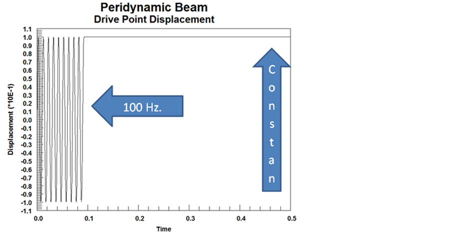
Figure 6. Driven end point transverse displacement.

Figure 7. Beam midpoint transverse displacement response.
The denser grid produces the same static solution as the coarse grid with a fixed horizon as shown in Figure 11.
4. Numerical Approach for Mixed Boundary Conditions
The application of Neumann boundary conditions in problems formulated with peridynamic theory can be problematic. Various authors have adopted approaches using boundary regions where the loading is specified in terms of body forces which are interior to the physical domain [12] or approaches where a hypothesized exterior
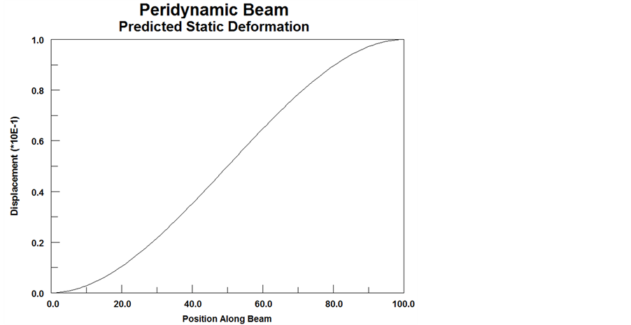
Figure 8. Beam midpoint transverse displacement response.
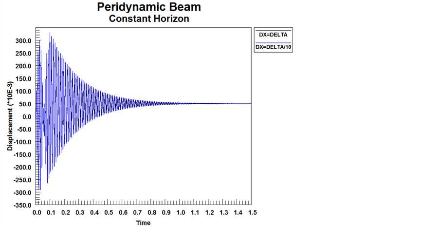
Figure 9. Center point transverse deflection for 2 grid spacings with constant δ.
domain is used as an extension of the physical domain [10] . Problems with Neumann conditions have also been treated by developing “compensation factors” accounting for the softening of the boundary [5] . All of these approaches require some assumption of smoothness in the boundary regions and/or iterative techniques [9] .
For the problem of the Timoshenko beam with mixed Dirichlet and Neumann boundary conditions, the approach taken here is to discretize the domain into cells of dimension Δ with a collocation point (or node) taken at the center of the cell. If the beam length is L, there are n = L/Δ cells in the domain. The horizon must include 3 or more cells and is fully consistent with the formulation given in Section 3. The equations of motion given in (36) and (37) are unchanged but a body force term must be included in the region of Neumann loading which approximates point load conditions. The solution procedure follows the Leapfrog-Verlet approach of Section 3, including the forces from loaded cells in the governing equations.
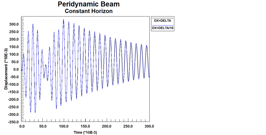
Figure 10. Early time response for fixed horizon with 2 grid spacings.

Figure 11. Predicted static deflection with constant horizon and 2 mesh densities.
Consider the case of an end loaded cantilever beam shown in Figure 12.
The left end of the beam (x = 0) is fixed (w = 0; γ = 0). The loaded end of the beam is approximated by adding a body force distributed in the end cell of the beam with value b = p/(AΔ) and the absence of a body moment. Ghost cells are added to integrate the peridynamic kernels beyond the physical domain using analytic continuation assuming smoothness of the variables. This is done using standard Taylor series expansions in the form:
 (53)
(53)
For the example problem given ahead, 2nd order finite differences are used to approximate the derivatives at the beam ends (backward differences at x = L and forward differences at x = 0). For the simple problem, using a first order Taylor series provided essentially identical results to problems solved with a 2nd order Taylor series. For more complex problems, higher order Taylor series extrapolations for analytical continuation may yield

Figure 12. Cantilever Beam with Free End Shear Loaded and Moment Free.
higher accuracy.
As an example problem, consider a beam with the parameters shown in Table 1 (example problem shown schematically in Figure 12):
The problem was solved assuming horizons of 2Δ, 3Δ and 4Δ. The load was applied as a step function and the solution was continued to steady state including the same damping applied in Section 3. The resulting static deflection curve is shown in Figure 13 and compared with the analytical solution. The peridynamic solution is almost identical to the analytic solution.
5. Discussion
The general motion of a micro-elastic beam undergoing infinitesimal deformations is found from the superposition of axial extension due to the axial load component, bending about the 2 planar axes of the beam cross-section and torsion about the axial direction. Sections 2-4 provide the solution process for all but the torsional deformation. If we restrict the discussion to non-warping torsional deformation, the micro-potential can be written as:
 (54)
(54)
where:
 (55)
(55)
with θ as the torsional twist angle. The corresponding peridynamic moment (the torsional moment) therefore, is:
 (56)
(56)
This is the same functional form as for the axial deformation of the peridynamic rod and the equations of motion are analogous to equation (1). The solution for torsion, therefore, follows the identical procedure as used for solution for axial deformation.
Sections 2 through 5 of this paper, therefore, provide the framework for the general solution of the fully three dimensional deformation of a micro-elastic Timoshenko beam under arbitrary loading (within the confines of beam theory).
6. Conclusions
Numerical predictions of the dynamic behavior of large, complex structures under load, are typically performed using beam, plate and shell assumptions in order to reduce the dimensionality of the analysis due to practical computing limitations. To take advantage of the strengths of the peridynamic solution methodology, therefore, it is necessary to develop and evaluate the peridynamic formulation for these structural elements. This paper provides the general formulation for the deformation of a Timoshenko beam using peridynamics. Numerical procedures are developed and are applicable to problems involving both Dirichlet and Neumann boundary conditions. For all cases studied, the damped dynamic peridynamic solutions converge to the solutions derived from Classical Continuum Mechanics (CCM). The characteristic dispersion introduced by peridynamics is noted in the dynamic solutions as has been discussed by various authors (e.g. [2] ). The paper provides both a theoretical and numerical approach which models deformations including rotational DOF and transverse shear effects. Work is ongoing to extend the approach to address peridynamic plates and shells in order to model the behavior of large thin-walled structures.
In the extension to plates and shells, the formulation will explore the use of State Based peridynamics as discussed in [3] [7] . This will facilitate the modeling of inelastic deformation states as well as finite deformation

Table 1. Beam parameters.
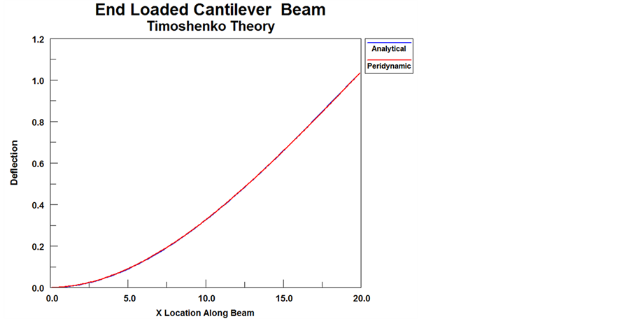
Figure 13. Comparison between the peridynamic and analytical solution for a cantilever beam with end loading.
processes. Finally the formulation will be packaged for inclusion in general purpose finite element codes. It is anticipated that solutions using peridynamic formulations will be computationally more expensive compared to finite element solutions for problems without fracture processes. Because of the advantages of the peridynamic approach for modeling material failure, the goal is to develop a peridynamic element which can be readily embedded in a finite element grid where fracture processes are predicted to occur. It is envisioned that a hybrid finite element-peridynamic solution for the modeling of crack propagation problems in large structures may provide an optimal solution procedure and combine the advantages of both computational approaches.
Acknowledgements
The authors would like to acknowledge the support from the In-House Laboratory Independent Research (ILIR) program at the NSWC Carderock Division, funded by the Office of Naval Research
References
- Silling, S.A. (2000) Reformulation of Elasticity Theory for Discontinuities and Long-Range Forces. Journal of the Mechanics and Physics of Solids, 83, 1526-1535.
- Emmrich, E. and Weckner, O. (2006) The Peridynamic Equation of Motion in Non-Local Elasticity Theory. III European Conference on Computational Mechanics: Solids, Structures and Coupled Problems in Engineering, Springer, Lisbon.
- Silling, S.A. and Lehoucq, R.B. (2010) Peridynamic Theory of Solid Mechanics. Sandia National Laboratory Technical Report SAMD 2010-1233J.
- Emmrich, E., Lehoucq, R.B. and Puhst, D. (2013) Peridynamics: A Nonlocal Continuum Theory. Meshfree Methods for Partial Differential Equations VI: Lecture Notes in Computational Science & Engineering, 89, 45-65. http://dx.doi.org/10.1007/978-3-642-32979-1_3
- Kilic, B. (2008) Peridynamic Theory for Progressive Failure Prediction in Homogeneous and Heterogeneous Materials, Ph.D. Thesis, University of Arizona, Tucson.
- Agwai, A. (2011) A Peridynamic Approach for Coupled Fields. Ph.D. Thesis, University of Arizona, Tucson.
- Tupek, M.R., Rimoli, J.J. and Radovitzky, R. (2013) An Approach for Incorporating Classical Continuum Damage Models in State-Based Peridynamics. Computational Methods in Applied Mechanical Engineering, 263, 20-26. http://dx.doi.org/10.1016/j.cma.2013.04.012
- Weckner, O. and Abeyarante, R. (2005) The Effect of Long-Range Forces on the Dynamics of a Bar. Journal of the Mechanics and Physics of Solids, 53, 705-728. http://dx.doi.org/10.1016/j.jmps.2004.08.006
- Duangpanya, M. (2011) A Peridynamic Formulation for Transient Heat Conduction in Bodies with Evolving Discontinuities. Ph.D. Thesis, University of Nebraska-Lincoln, Lincoln.
- Bobaru, F., Yang, M., Alves, L.F., Silling, S., Askari, E. and Xu, J. (2009) Convergence, Adaptive Refinement, and Scaling in 1D Peridynamics. International Journal for Numerical Methods in Engineering, 77, 852-877. http://dx.doi.org/10.1002/nme.2439
- Feynman, R.P., Leighton, R.B. and Samds, M. (1963) Chapter 9, Newton’s Laws of Dynamics. The Feynman Lectures on Physics, 1, Addison-Wesley.
- Demmie, P.N. and Silling, S.A. (2007) An Approach to Modeling Extreme Loading of Structures Using Peridynamics. Journal of Mechanics of Materials and Structures, 2, 1921-1945. http://dx.doi.org/10.2140/jomms.2007.2.1921