Direct Calculation of Unsteady-State Weymouth Equations for Gas Volumetric Flow Rate with Different Friction Factors in Horizontal and Inclined Pipes

doi:10.4236/eng.2012.44027

Engineering
Vol. 4 No. 4 (2012) , Article ID: 18828 , 8 pages DOI:10.4236/eng.2012.44027

Abayomi O. Olatunde¹, Tunde A. Adeosun^2*, Mohammed A. Usman¹, Olabisi M. Odunlami³, Moses A. Olowofoyeku⁴, Testy E. Ekakitie², Atanda M. Mohammed²

●How to Cite this Article

¹Department of Chemical Engineering, University of Lagos, Lagos, Nigeria

²Department of Mathematics, Yaba College of Technology, Yaba, Nigeria

³Department of Chemical Engineering, Lagos State Polytechnic, Lagos, Nigeria

⁴Department of Civil Engineering, Yaba College of Technology, Yaba, Nigeria

Email: ^*adebaba2001@yahoo.com

Received January 26, 2012; revised March 7, 2012; accepted March 15, 2012

Keywords: Unsteady-State; Flow Rate; Friction Factor; Stability; Variations; Unsteadiness

ABSTRACT

Direct calculations of unsteady-state Weymouth equations for gas volumetric flow rate occur more frequently in the design and operation analysis of natural gas systems. Most of the existing gas pipelines design procedures are based on a particular friction factor and steady-state flow analysis. This paper examined the behavior of different friction factors and the need to develop model analysis capable of calculating unsteady-state gas flow rate in horizontal and inclined pipes. The results show different variation in flow rate with Panhandle A and Panhandle B attaining stability in accurate time with initial unsteadiness at the instance of flow. Chen and Jain friction factors have opposition to flow with high flow rate: The prediction also reveals that Colebrook-White degenerated to Nikuradse friction factor at high Reynolds number. The horizontal and inclined flow equations are considerably enhanced on the usage of different friction factors with the aid of Matlab to handle these calculations.

1. Introduction

[1] derived gas flow equation in a rigorous algebraic analytical equation for isothermal steady-state flow in gas pipeline to calculate volumetric flow rate and pressure losses in horizontal pipelines. For slightly inclined pipes, the elevation change is compensated by simply adding the static head of gas column to the pressure losses. Researchers continue to develop transient mathematical models that focus on the unsteady nature of these systems. Many related design problems, however, could be solved using steady-state modeling. Several investigators have studied the problem of gas flow through the pipeline and have developed a range of numerical schemes, which include the method of characteristics, finite element methods, and explicit and implicit finite difference methods. The choice partly depends on the individual requirements of the system under investigation. Common solution techniques for steady-state network analysis include nodal and loop formulation [2] and the entire set of hydraulic equation [3]. Reference [4] presented a central implicit finite difference method and compared this method with the method of characteristics. They showed that the implicit method is very accurate for large time steps and so in the implicit procedure the maximum practical time increment is limited by the frequency of the variables imposed at the boundary condition at the inlet and outlet ends of the pipe. [5,6] discussed the importance of a transient simulation and the advantages of using a transient simulation. He notes that transient simulation is not only an excellent tool for training operations personnel, but it can also act as a helpful tool in on-line systems. He emphasizes its use in the design phase of a gas pipeline without storage facilities and with a flow demand that varies with respect to time on an hourly basis so as to show a behavior that could not be considered as a steady state.

[7,8] compared a variety of transient models. Numerical solution of the partial differential equations, which characterize a dynamic model of the network, requires significant computational resources. The problem is to find, for a given mathematical model of a pipeline, a numerical method that meets the criteria of accuracy and relatively small computation time. The main goal of this paper is to characterize different transient models and existing numerical techniques to solve the transient equations. Reference [9] presented an analytical unsteadystate flow equation for gas pipelines in two categories: gas flow in wellbore during production and gas flow in pipe-lines during transportation. This is the most recent development that was based on the steady-state gas flow developed [10], and the paper assumed Moody friction factor and observed in their paper that all unsteady-state processes tend towards steady-state with time and applicable over a wide range of Reynolds number and relative roughness values within an acceptable standard of accuracy. The methods for gas pipeline calculations have some limitations in their accuracy due to assumptions considered in the used of friction factors on their models. Most of the methods neglected kinetic energy contribution. All are developed on the basis of steady-state flow for horizontal and inclined pipes. Most recently, [11] developed equations that assume unsteady-state gas volumetric flow rate calculations that are based on Weymouth’s equations. The new equations are obtained by solving the fundamental energy equation without neglecting any assumption in the momentum equation. However, the basic flow equation consists of four components: elevation, kinetic energy, frictional losses and accumulation term. The elevation component is dependent upon the gas gravity and when computed over the length of a horizontal or inclined pipeline becomes negligible.

In this work, the developed model equations in [11] will be applied to other friction factor equations producing different flow rate from the unsteady-state Weymouth equations. Use of fundamental equation for calculating flow requires the numerical evaluation of friction factor. In general the friction factor itself is in turn a function of flow rate, thus making the whole flow equation an implicit one. For the purpose of determining friction factor, it has been found that fluid flow may be characterized by a dimensionless grouping of variables known as Reynolds number. The other parameter in the friction factor correlation is pipe roughness. Friction factor may be correlated as a function of the Reynolds number and the relative pipe roughness. Reynolds numbers are defined as the ratio of gas density, gas velocity, and pipe diameter to gas viscosity. The relative roughness is expressed as the absolute roughness of the pipe to its diameter.

This paper considered different friction factor equations for use in Equations (1) and (2) and these are substituted into the unsteady state equations for solutions. These solutions can be used to calculate the instantaneous volumetric gas flow rate in both horizontal and inclined pipes if p₁ and p₂ are known. The developed equations for both the horizontal and incline pipes are stated as follows:

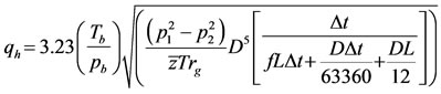(1)

for horizontal pipeline and

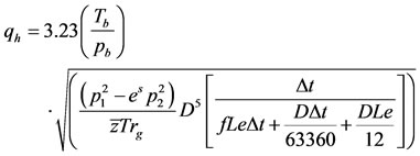(2)

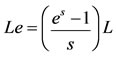
For vertical pipeline. For a uniform slope:

where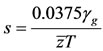

and if the Moody friction factor for Weymouth equation is

(3)

All these friction factors below will be substituted into Equations (1) and (2) respectively to calculate the instantaneous volumetric gas flow rate in horizontal and inclined pipes.

1.1. Panhandle A Equation

The Panhandle A pipeline flow equation assumes that f varies as follows:

(4)

1.2. Panhandle B Equation

This is probably the most widely used equation for long lines (transmission and delivery). The modified Panhandle equation assumes that f varies as

(5)

1.3. Nikuradse’s Friction Factor

This correlation is still the best one available for fully developed turbulent flow in rough pipes:

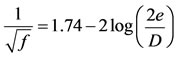(6)

1.4. Hagen-Poiseuille Equation

This is used for laminar flow.

(7)

1.5. Chen Equation

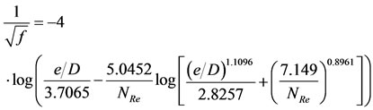(8)

1.6. Jain Equation

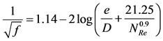(9)

1.7. Colebrook-White Equation

This is applicable to smooth pipes and to flow in transition and fully rough zones of turbulent flow.

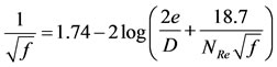(10)

2. Analysis of the Unsteady-State Analytical Equation

Equations (1) and (2) are for horizontal and inclined pipes and these provide a fundamental relationship between gas flow rate, inlet and outlet pressures, and the usual pipeline parameters. These two equations are based on fundamental fluid flow equations that governs compressible gas flow in pipes [9-14] considered a single phase real gas flow in pipe with uniform cross-sectional area using the mass conservation principle to developed a conservation equation for a control system that includes energy equation that so obtained the unsteady-state equations for gas flow in pipes and these can be applied to a variety of problems.

In deriving Equations (1) and (2), it was assumed that temperature and compressibility factor are constant, for a very short piece of pipeline, this assumption claimed to be valid and thus the equations should be accurate [11]. These equations can be used to estimate any of these variables in the specified order. However, we can always divide a long pipeline into small segments for stepwise calculations to retain the same level of accuracy.

3. Result and Discussions

The volumetric gas flow rate for horizontal and inclined pipes is calculated for a period of 1000 hours using Equations (1) and (2) for the different friction factors. These are compared with steady-state gas flow for both horizontal and inclined pipes and are hereby discussed. Figure 1 shows the variation of flow rate with time for both horizontal and inclined pipes using Panhandle A Equation. The graph shows increase in the flow rate from 0 to 380 hours and stabilizes from 400 to 1000 hours for horizontal pipe. It also shows increase in flow rate from 0 to 560 hours and then stabilizes from 580 to 1000 hours for inclined pipe. The steady state gas flow rate is achievable as 49.4 MMScf/hour for horizontal pipe and 38.2 MMScf/hour for inclined pipe. Figure 2 shows the variation of flow rate with time for both horizontal and inclined pipes using Panhandle B Equation. The graph shows increase in the flow rate from 0 to 420 hours and then stabilizes from 440 to 1000 hours for horizontal pipe. The graph shows that the flow rate also increases from 0 to 480 hours and then stabilizes from 500 to 1000 hours for inclined pipe.

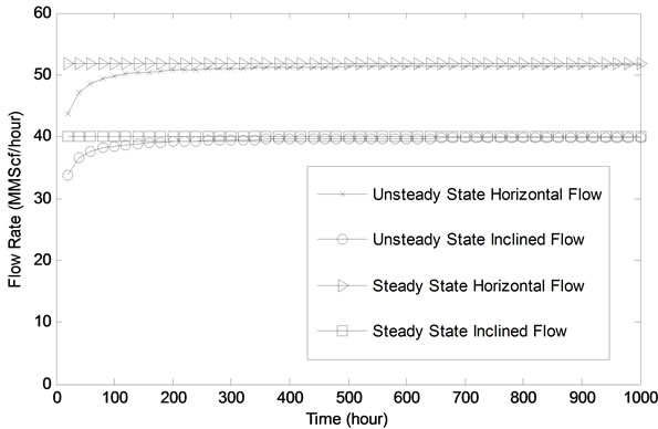
Figure 1. Flow rate variation with time using Panhandle A Equation.

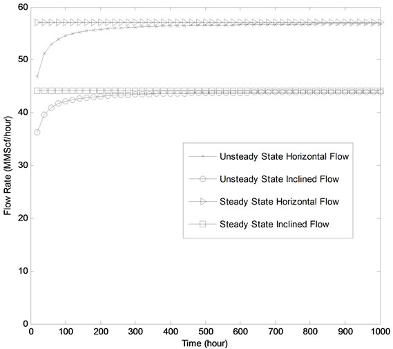
Figure 2. Flow rate variation with using Panhandle B Equation.

The steady-state gas flow rate is achievable as 56.5 MMScf/hour for horizontal pipe and 43.7 MMScf/hour for inclined flow. Figure 3 shows the variation of flow rate with time for both horizontal and inclined pipes using Nikuradse’s friction factor. The graph shows increase in the flow rate from 0 to 420 hours and then stabilizes from 440 to 1000 hours for horizontal pipe. The graph shows that the flow rate also increases from 0 to 680 hours and then stabilizes from 700 to 1000 hours for inclined pipe. The steady-state gas flow rate is achievable as 40.2 MM Scf/hour for horizontal pipe and 31.1 MMScf/hour for inclined pipe. Figure 4 shows the variation of flow rate with time for both horizontal and inclined pipes using Hagen-Poiseuille Equation. The graph shows increase in the flow rate from 0 to 380 hours and then stabilizes from 400 to 1000 hours for horizontal pipe. The graph shows that the flow rate also increases from 0 to 420 hours and then stabilizes from 440 to 1000 hours for inclined pipe. The steady-state gas flow rate is achievable as 59.2 MM Scf/hour for horizontal pipe and 45.8 MMScf/hour for inclined pipe. Figure 5 shows the variation of flow rate with time for both horizontal and inclined pipes using Chen Equation. The graph shows increase in the flow rate from 0 to 680 hours and then stabilizes from 700 to 1000 hours for horizontal pipe. The graph also shows increase in flow rate from 0 to 920 hours and then stabilizes from 940 to 1000 hours for inclined pipe.

The steady-state gas flow rate is achievable as 79.0 MMScf/hour for horizontal pipe and 61.1 MMScf/hour for inclined pipe. Figure 6 shows the variation of flow rate with time for both horizontal and inclined pipes using Jain Equation. The graph shows increase in the flow rate from 0 to 640 hours and then stabilizes from 660 to 1000 hours for horizontal pipe. The graph shows that the flow rate also increases from 0 to 680 hours and then stabilizes from 700 to 1000 hours for inclined pipe.

The steady-state gas flow rate is achievable as 39.5 MMScf/hour for horizontal pipe and 30.5 MMScf/hour for inclined pipe. Figure 7 shows the variation of flow rate with time for both horizontal and inclined pipes using Colebrook-White Equation. The graph shows increase in the flow rate from 0 to 440 hours and then stabilizes from 460 to 1000 hours for horizontal pipe. The graph shows that the flow rate also increases from 0 to 740 hours and then stabilizes from 760 to 1000 hours for inclined pipe. The steady-state gas flow rate is achievable as 40.2 MMScf/hour for horizontal pipe and 31.0 MMScf/hour for inclined pipe.

The analysis of results and discussion shows that all the flow variations in the graphs are evident that there exists an initial transience at the instance of flow which later stabilizes with time. It is observed that the flow rate for inclined flow is smaller when compared to horizontal flow. It is also observed that it took a longer time to achieve steadiness in inclined pipes as compared to horizontal pipes and these observations can be attributed to gravity effect due to change in elevation. The gas volumetric

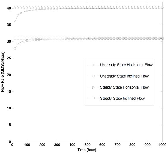
Figure 3. Flow rate variation with time using Nikuradse’s friction factor.

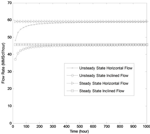
Figure 4. Flow variation with time using Hagen-Poiseuille Equation.

flow rate obtained when using Panhandle B is higher than the volumetric flow rate when using Panhandle A.

This can be attributed to the fact that Panhandle B equation is correlated for higher flow rates. We also observed that gas volumetric flow rate increased with decreasing friction factor.

Chen Equation which has a friction factor of 0.0045 has the highest flow rate while Jain Equation which has a friction factor of 0.01739 has the lowest flow rate. This can be attributed to friction factor that shows the degree

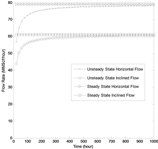
Figure 5. Flow variation with time using Chen Equation.

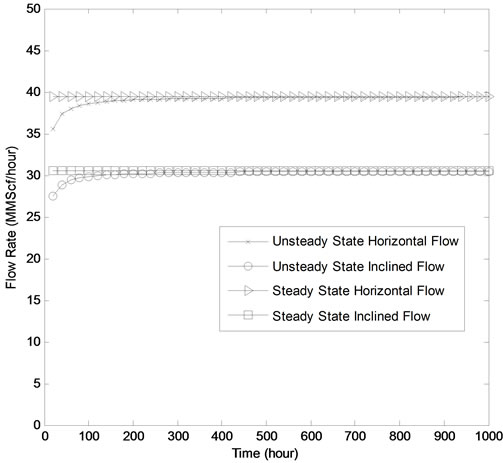
Figure 6. Flow variation with time using Jain Equation.

to which flow is opposed in a pipe. Hence, a small friction factor means that opposition to flow is low which implies high flow rate and vice versa.

The Nikuradse’s friction factor obtained is approximately equal to the friction factor of the ColebrookWhite Equation for a Reynolds number of 8 × 10⁵. This is because Colebrook-White degenerates to Nikuradse correlation at high Reynolds number.

4. Conclusion

Direct calculation of unsteady-state Weymouth equations has been examined on different friction factors without

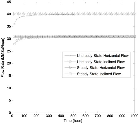
Figure 7. Flow variation with time using Colebrook-White Equation.

neglecting any of the terms in the fundamental gas flow equations. These friction factors show a functional relationship between flow rate, inlet and outlet pressure and are very useful in gas pipeline calculations where any of these variables needs to be estimated if the others are given. The friction factors show different variation in flow rate with more realistic results, however, we can predict that panhandle A and panhandle B are more accurate in attaining stability with initial unsteadiness and flow rate at any given time. It is observed that Chen and Jain friction factors have opposition to flow which implies high flow rate and vice versa. The examination also observed that Colebrook-White degenerate to Nikuradse friction factor at high Reynolds number. In conclusion, we observed that all unsteady-state processes tend towards steady-state with time. The initial unsteadiness at the instance of flow is enhanced at high Reynolds number. The usage have tremendous application when examined through different friction factors and is able to predict unsteady-state flow in pipeline compare to the steady-state process assumed in industry.

5. Acknowledgements

The authors acknowledged the support of the Chemical Engineering lab at the University of Lagos and the assistance and suggestions. Authors would like to thank the Nigerian Gas Company for making it possible to write this paper.

REFERENCES

T. R. Weymouth, “Problems in Natural Gas Engineering,” Transactions of the ASME, Vol. 34, 1912, p. 185.
J. A. Ferguson, “Gas Flow in Long Pipelines,” Chemical Engineering, Vol. 56, No. 11, 2002, pp. 112-135.
M. A. Stoner, “Steady-State Analysis of Gas Production, Transmission and Distribution Systems,” Fall Meeting of the Society of Petroleum Engineers of AIME, Denver, 28 September-1 October 1969, 8 Pages.
D. W. Schroeder, “A Tutorial on Pipe Flow Equations,” 33rd Annual Meeting Pipeline Simulation Interest Group (PSIG), Salt Lake City, 17-19 October 2001.
J. Zhou and M. A. Adewumi, “Gas Pipeline Network Analysis Using an Analytic Steady-State Flow Equation,” Eastern Regional Meeting, Pittsburgh, 9-11 November 1998, 13 Pages.
L. Ouyang and K. Aziz, “Steady-State Gas Flow in Pipes,” Journal of Petroleum Science and Engineering, Vol. 14, No. 3-4, 1996, pp. 137-158. doi:10.1016/0920-4105(95)00042-9.
R. N. Maddox and P. Zhou, “Use of Steady-State Equations for Transient Flow Calculations,” 15th Annual Meeting Pipeline Simulation Interest Group (PSIG), Detroit, 27-28 October 1983.
G. A. Rhoads, “Which Flow Equation—Does It Matter?” 15th Annual Meeting Pipeline Simulation Interest Group (PSIG), Detroit, 27-28 October 1983.
T. A. Adeosun, A. O. Olatunde and A. Okwananke, “Development of Unsteady-State Equations for the Flow of Gas through Pipelines,” Journal of Advances and Applications in Fluid Mechanics, Vol. 7, No. 1, 2010, pp. 45-60.
S. Tian and M. A. Adewumi, “Development of Analytical Design Equation for Gas Pipelines,” SPE Production & Facilities, Vol. 9, No. 2, 1994, pp. 100-106.
T. A. Adeosun, A. O. Olatunde, J. O. Aderohunmu and T. O. Ogunjare, “Development of Unsteady-State Weymouth Equations for Gas Volumetric Flow Rate in Horizontal and Inclined Pipes,” Journal of Natural Gas Science and Engineering, Vol. 1, No. 1, 2009, pp. 113-117. doi:10.1016/j.jngse.2009.09.001
D. L. Katz and R. L. Lee, “Natural Gas Engineering Production and Storage,” McGraw-Hill Publishing Co., New York, 1990.
C. U. Ikoku, “Natural Gas Production Engineering,” John Wiley and Sons Publishing Co, New York, 1984.
P. U. Ohirihian, “Direct Calculation of the Gas Volumetric Flow Rate in Horizontal and Inclined Pipes,” Paper SPE 37394, 2002.