Intelligent Control and Automation
Vol.4 No.2(2013), Article ID:31737,12 pages DOI:10.4236/ica.2013.42020
A Tree-Type Memory Formation by Sensorimotor Feedback: A Possible Approach to the Development of Robotic Cognition
1Brain Science Institute, RIKEN, Nagoya, Japan
2Department of Human and Artificial Intelligence Systems, Fukui, Japan
Email: fady@synapse.his.u-fukui.ac.jp
Copyright © 2013 Fady Alnajjar et al. This is an open access article distributed under the Creative Commons Attribution License, which permits unrestricted use, distribution, and reproduction in any medium, provided the original work is properly cited.
Received August 6, 2012; revised January 28, 2013; accepted February 7, 2013
Keywords: Visiomotor Abstraction; Memory Based Learning; Artificial Cognition; Internal Representation
ABSTRACT
Based on indications from neuroscience and psychology, both perception and action can be internally simulated in organisms by activating sensory and/or motor areas in the brain without actual external sensory input and/or without any resulting behavior (a phenomenon called Thinking). This phenomenon is usually used by the organisms to cope with missing external inputs. Applying such phenomenon in a real robot recently has taken the attention of many researchers. Although some work has been reported on this issue, none of this work has so far considered the potential of the robot’s vision at the sensorimotor abstraction level, where extracting data from the environment takes place. In this study, a novel visiomotor abstraction is presented into a physical robot through a memory-based learning algorithm. Experimental results indicate that our robot with its vision could develop a kind of simple anticipation mechanism into its tree-type memory structure through interacting with the environment which would guide its behavior in the absence of external inputs.
1. Introduction
Real world applications are usually subject to change and very difficult to be predicted. Any sudden changes in the environment can possibly cause temporary lose in communication with the external world. Some organisms, those that have the ability of cognition or thinking, can cope with such situations by replacing the external missing or corrupted sensory data with their own internal representation (or experience).
In recent decades, a branch of science called cognitive neuroscience, an interdisciplinary link between cognitive psychology and neuroscience, has been established to introduce such phenomena to the mobile robot [1]. It was hoped that adding this feature to the robot would move autonomous robots closer to interfacing with real world applications.
Cognitive Roboticsis concerned with endowing robots with mammalian and human-like cognitive capabilities to enable them to accomplish complex tasks in complex environments. Cognitive ability is the ability to understand and try to make sense of the world. In [2], the authors have argued that all living creatures are cognitive to some degree. Several authors have argued in recent years that cognition and consciousness can be achieved to some extent on the mobile robots [3-5]. We believe that the level of or how much the robot could be conscious of the surrounding environment depends on how much the robot knows about this environment. Cognition in robots includes perception processing, attention allocation, anticipation, etc. One of the possible approaches to measuring these capabilities in the robot is by examining its ability to cope with missing external sensory data during performance of a specific task. Said in a different and operational way, it is the ability of a robot to perform blindfolded navigation, where the robot navigates within a known environment using only its internal representation.
In recent years, building a complete blindfolded navigation system in a mobile robot has been a challenging task for many robotic researchers [6-9]. For instance, some initial experiments were presented in [7] that aim to contribute toward building a robot that navigates completely blindfolded in a simple environment using a two-level network architecture; 1) low-level abstraction from sensorimotor values to a limited number of simple abstract “concepts”, following the work done by Linker and Niklasson [6,10], and 2) higher-level prediction/ representation of the agent’s interaction with the environment, inspired by the work done by Nolfi and Tani [11]. These efforts have to some degree succeeded in allowing the robot to anticipate long chains of future situations. However, they have failed to support a completely blindfolded navigation [8], in which the robot repeatedly uses its own internal representation values instead of the real sensory inputs for a certain number of times for its navigation. The failure partly seems to be due to the short range of the robot’s proximity sensors that they used, which limits the amount of data that could be abstracted from the environment. The consequence of this limitation is that the robot does not have enough sensitivity about the environment. We argue here that improving the robot’s sensorimotor abstraction level, therefore, could possibly overcome this problem. For instance, instead of relying only on the limited data provided by the robot proximity sensors, let the robot see the environment using its camera, abstract enough data, and arrange it well in its memory to aid in building its internal representation.
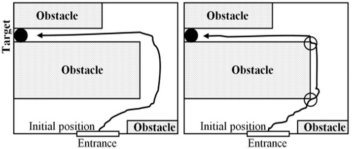
To support our argument, we have done psychological experiments, similar to the one introduced by Lee and Thompson [12] with a little change. In a series of two experiments, we demonstrated the accuracy with which humans can guide their behavior based only on their internally sensory experiences. Two subjects were asked to do the same task under different conditions. The first subject X was asked to “look” around in a given room and locate a specific target (Figure 1(a)). He was then blindfolded and asked to locate the target again. The subject performed the task accurately with closed eyes, in the same manner as when he was free to “look” (Figure 1(b)). However, he could not predict the exact time needed to turn to the target and this caused the two hits with the obstacle (the empty circles in Figure 1(b)). The second subject Y was not allowed to explore the room with his eyes (no vision input). Instead, he was blindfolded and walked around the room touching things around him until he found the target (Figure 1(c)). He was then asked to seek the target again blindfolded from the initial position. Though successful in reaching the target, he took more time than that needed by subject X. In addition, the number of times that he hit the wall or touched it to correct or locate his direction was greater (Figure 1(d)).
From the above experiment we can conclude that subject X had collected a sufficient amount of data from the environment during his first “eyes open” navigation. This data could be various dimensions in the room which the
 (a)
(a) (b)
(b)
Figure 1. The track of subject X in the first case: (a) Eyes were opened; (b) Eyes were closed. The track of the subject Y in the second case (closed eyes); (c) The first try to reach the target; (d) The second try. The empty circles present the places where the agent was using the wall to correct or locate his position.
subject related to times and distances that helped him to build internally—in his inner world where sensory experiences and consequences of different behaviors may be anticipated—his own internal image. In contrast, the amount of data that subject (Y) had collected was limited to the objects that his hand touched during his first blindfolded navigation and their relation to his moving steps. This data, however, was not good enough to accurately perform the task.
In the above experiment, subject Y could be a demonstration of the results of the most recently reported works (e.g., [7]), since they used the short-range proximity sensors for building the sensorimotor abstraction level.
We also tried to demonstrate the inner world that was automatically built inside both subjects’ memory by giving each of them a sheet of white paper and asking them to draw the outline of the room that they trained in (note that subject Y had never seen the room). It was not surprising to find out that subject X could draw almost all the details of the room (Figure 2(a)). However, subject Y could hardly draw the layout of just the objects that he touched during his movement (Figure 2(b)).
The work presented in this paper was motivated by the problems described above. Here we explore the inner world of a real mobile robot that has a chance to explore the surrounding environment with its camera before it was told to navigate blindfolded in it. In this study, the robot used two network architectures. The first was used to control its navigation, while the second, to build its internal representation.
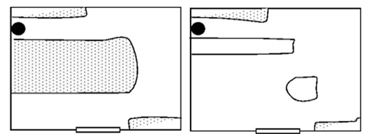
Figure 2. (a) and (b) illustrate the environment as it is perceived “imagined” by subjects X and Y, respectively.
2. Background
A number of researchers have tried to investigate the robot’s internal representation or as it called by some; the robot’s inner world [5,13]. In [5], for instance, the author describes development of three simulation hypotheses in order to explain the robot’s inner world. This was also discussed by Stening in [7]; and we summarized it in this section. The first is covert behavior, which is the ability to generate internally neural motor responses that are not actually externally executed. The second is sensor imagery, which is the ability to internally activate the sensory areas in the brain, so as to produce the simulated experience without actual external inputs. The third is anticipation, which is the ability to predict the sensory consequences of the motor response. More information regarding each assumption is given by [5,7].
Based on the above hypotheses, the internal sequences of the robot behaviors could be illustrated by Figure 3. In Figure 3(a), a situation S1 elicits internal activity s1, which in turn leads to a motor response preparation r1 and thereafter results in the overt behavior R1, which causes a new situation S2. In Figure 3(b), because of the robot’s past experiences, the response preparation r1 could directly elicit the internal activity s2. In Figure 3(c), if the robot trains the network to some degree, then it should be possible to simulate long sequences of motor responses and sensory consequences.
Several modelers have translated the ideas shown in Figure 3(c), directly into the robot [7]. From the figure, these modelers (Figure 3(d) for an example) have not only mapped the sensory input to motor output but also predicted the next time step’s sensory input based on the network’s experience with the environment, which is stored in a kind of a short-term memory that is then used instead of the real one in each time step.
Much of the later work has been following a similar basis, e.g. [14-16]. All of these studies, however, have considered only the robot’s short-range proximity sensors (e.g., IR sensor) in their experiments, which therefore, cannot provide enough data about the environment for the robot to build its internal representation.
From the psychological experiments reported in the
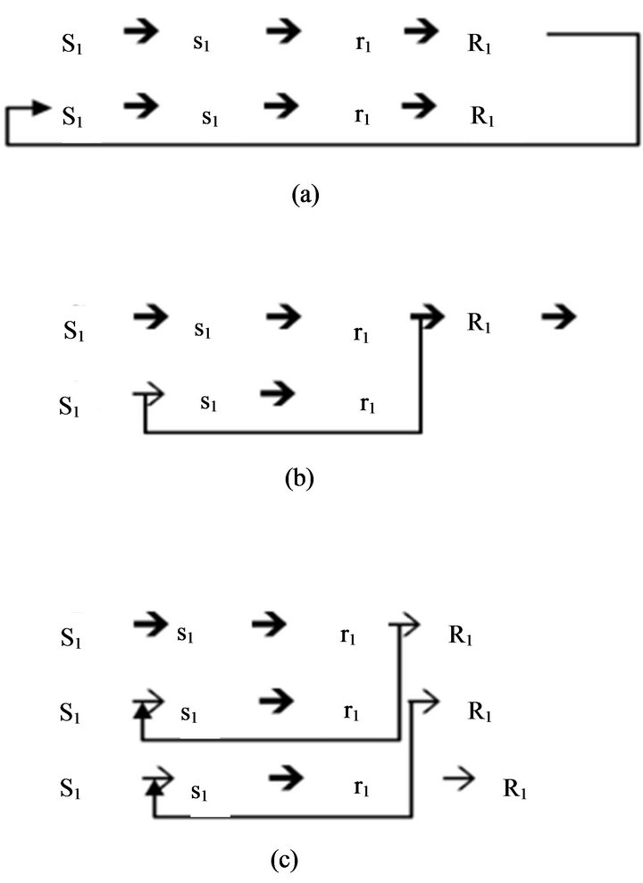

Figure 3. (a)-(c) The basic principle of Hesslow’s simulation hypothesis (adopted from [5]); (d) The basic approach to simulation of perception in robots used by [7,13].
previous section, we agree with [4,5,7] that the weak spot in simulation theories is concerning the matter of the abstraction level at which internal representation are relied on. Therefore, improving the ability of this level should result in building a better internal representation in the robot, and therefore, better cognition ability.
In this paper, we examine the possibility of a physical mobile robot using its vision to build an organized internal representation of a given environment sufficient for its blindfolded navigation.
3. Robot and Environment
All the experiments in this study were conducted in a physical mobile robot “Hemisson”. Hemisson is a miniature mobile robot that was originally developed for educational purposes by K-team (www.k-team.com) (Figure 4(a)). It is equipped with several IR sensors and a programmable 8bit MCU. The robot is able to avoid obstacles, detect ambient light intensity and follow a line on the floor. Other components are also included, such as a programmable LED, a buzzer, and switches. Hemisson is also equipped with a wireless camera module to transmit video images to a receiver that is connected to a PC for image processing.
As discussed earlier, we used the robot’s IR sensors to supply the sensory input in the first network, while the robot’s camera sensors were used to supply the second network. The robot’s camera view has been divided into 4 parts, as illustrated in Figure 4(c). Each part covers a number of pixels that represent the distance to the obstacles (by counting the number of white pixels from the lower edge of the image till the lower edge of the obstacle). We have applied the idea of flood fill algorithm [17] to filter the robot’s view and to easily clarify the boundaries between the floor and the obstacles. We arranged an ideal environment for the robot to navigate in to avoid a large amount of image processing, since image processing is not the main target of this work. The combination of these pixel parts was used to identify the current concept of the robot’s view CC. The average of FL and FR were used to calculate the real distance Dcm to the frontal obstacles. A simple neural network was trained by Back-Propagation algorithm (BP) to convert the number of pixels in each part into a real distance. The environment structure that we used was similar to the one used by [7,11], consisting of two different-sized rooms connected by a short corridor (Figure 4(b)).
4. Experiments
4.1. Proposed Architecture
The general network architecture presented in this study was inspired by the architecture presented in [7,13]. In their work, they used two-level neural network architectture. The lower level consisted of an unsupervised vector quantizer that categorized the current IR-sensory and motor values into a more abstract level they called “concepts”, such as “corner” or “corridor”. The higher level consisted of a recurrent neural network that trained to predict the sequence of lower-level concepts and their respective duration, (for example, following a right wall for 45 time steps would be followed by a left-turn corner that lasted for 3 time steps, etc.)
Our architecture, in contrast, differs from this previous
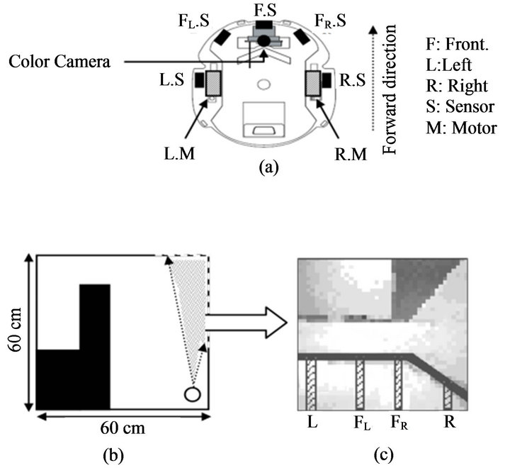
Figure 4. (a) Schematic drawing illustrates the position of the IR-Sensors, color camera and motors on Hemisson; (b) Robot environment. The empty circle illustrates the robot. The doted area illustrates the range of the robot’s view; (c) Robot’s view in the position shown in B. Black thick line illustrates the lower edge of the obstacle. The vertical lines L, FL, FR and R, illustrate the left, left-front, right-front and right pixels range reading, respectively.
work in two main aspects. First, instead of using only the robot’s IR sensors as an input for the abstract level, we added the robot’s vision sensors to the system. The second main difference is that the robot has two separated networks. The first network is used to control the robot’s navigation system within the environment, as shown in Figure 5(a). The second network represents the robot’s memory, as shown in Figure 5(b). It is used to abstract data from both the first network (motors’ speed) and the environment. It also learns the relationships between these data to build the robot’s internal representation, and to predict both the upcoming concept (PNC) and the time needed to go through each concept (PT).
We initially trained the second network with BP. However, the error ratio was high even when we trained the robot for a very long time. We also tried to evolve the network with standard Genetic Algorithm (GA), but unfortunately the results did not improve. The reasons for these failures could be one of the following. First, the number of concepts generated by the robot’s camera could have created a sequence which is too complex for such algorithms to learn. Second, we are dealing with a physical mobile robot that makes learning through these types of evolutionary algorithms quite impossible, since it may require several days to complete one experiment.
To try to get around this problem, we shifted the learning process in the second network so it was based on the contents of the robot’s memory, as inspired by the work
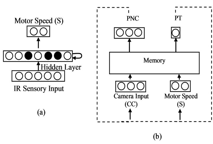
Figure 5. (a) Architecture of the SNN used in the first network. White/black circles represent excitatory/inhibitory neurons which have positive/negative connection, respecttively. The neurons in the hidden layer are fully connected to each other; (b) Architecture of the second network. PNC and PT are the output of the robot’s memory at each time step. The dashed line illustrates the connection that was done in experiment 4, where the outputs of the network were replaced with the real input values.
of [18] with small changes, i.e., while the robot is navigating in the environment using the first network, the second network predicts from its past experience, or randomly, what will be the next view or action, and then corrects its prediction layer by the actual fact when it faces it (See Figure 6 for an example). This algorithm turned out to be reasonably successful.
A tree-type memory structure has been introduced to the second network (robot’s memory), similar to the one introduced in [19] (Figure 7). This memory has a dynamic structure and simple storing and retrieving mechanism. It was also supported by forgetting and clustering mechanisms to control its general size and to provide maximum memorizing ability. More details can be found in [19]. The memory was divided into five levels. The first three levels were used to store the robot camera inputs to identify each concept. The fourth level (ε) was used to count the number of concepts in each environment, so as to identify the environment. The last level represents the prediction layer.
During the navigation, the robot built its memory based on its experiences and gradually learned from them for its future action. The flowchart in Figure 8 shows the working mechanism of the memory. According to the chart, when the robot returns to its straight state after performing the turning in the corridor or corner, two phases are operated sequentially: the learning phase, where the robot learns and updates its memory with the currently available facts, and the predicting phase, where the robot explores the environment and gradually builds its experiences. The following points briefly summarizeing the flowchart:
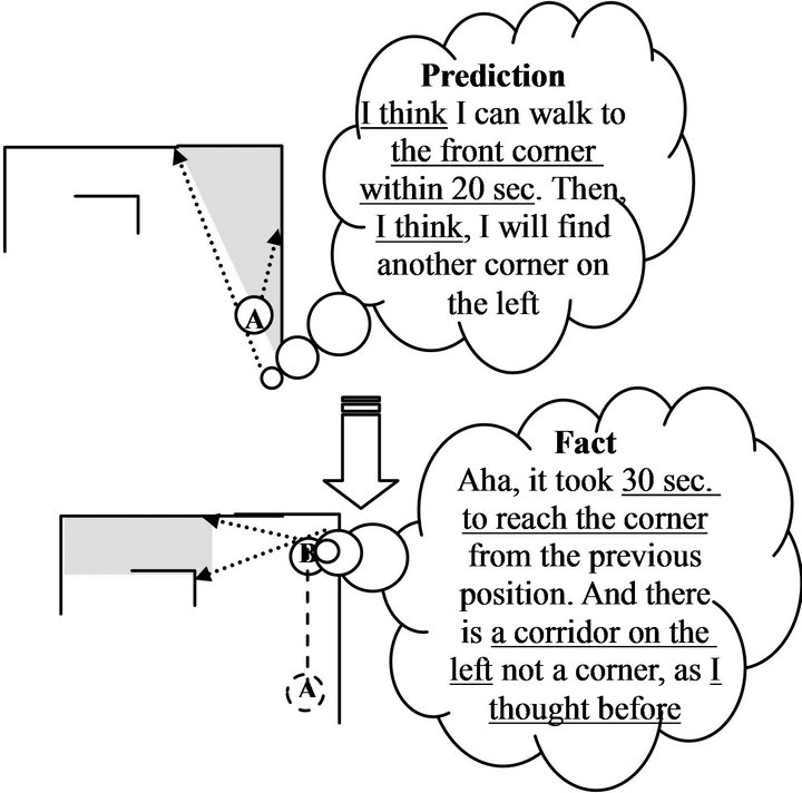
Figure 6. An example of how the robot’s memory builds and updates its knowledge.
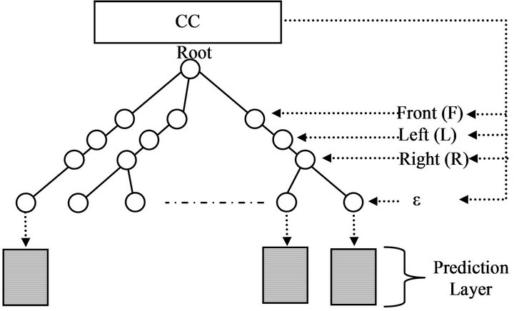
Figure 7. Tree-memory structure used in this study (adopted from [19]). Each concept has its own prediction layer, which contains PNC, PT and the end action of each concept, e.g., turns right (TR) or turns left (TL).
Learning phase (the thick lines in Figure 8):
• Robot takes a photo of its current view CC, finds the distance to the obstacle (D), finds its motor speed (S), and calculates PT (PT = D/S + α). Where (α) is the prediction time delay between the real time that the robot manually counts during its movement (RT) and the time that the robot predicts based on its experience (PT) (α = |RT − PT|).
• If the robot has previously predicted the current concept from the previous stage, i.e., the next concept buffer (NCB) is not empty, and RT contains the real time needed for the robot to finish the previous stage, then the robot needs to ascertain the validity of the previous stage’s prediction layer PNC, which also is stored in NCB, with the current concept.
• If the CC is equal to NCB, then the prediction layer of the previous stage is correct. Therefore the error prediction function (e) decreases, otherwise, it increases,
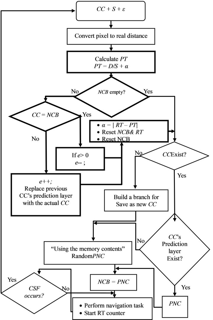
Figure 8. The working mechanism of the robot’s memory. Thick lines illustrated the learning phase, while thin lines illustrated the predicting phase.
i.e., the previous stage prediction layer PNC is incorrect and should be replaced by the current CC. The prediction time delay α is also updated by the current value of RT to adjust the value of PT.
Predicting phase (the thin lines in Figure 8):
• If the current concept CC does not exist in the robot’s memory, i.e., the robot has not seen the view before, a new branch will grow up in the memory to hold the value of the new CC.
• If the CC exists in the robot’s memory, then the robot’s history buffer ε and CC’s prediction layer are combined to predict the next concept PNC. Where (ε = ε + CC) if CC exists in ε queue, otherwise, (ε = ε – CC). If CC’s prediction layer has no experience about the next view, the memory will randomly choose a PNC from any existing data in the memory and store it in the NCB, which will be corrected later by the learning phase (step 2).
• The robot starts to perform wall-following behavior until the next activation of changing-state flag (CSF), i.e., whenever the robot returns to its forward position after finishing performing another action (e.g., turning right or left).
4.2. Experimental Results
4.2.1. First Stage (Wall-Following Behavior)
In order to control the robot’s initial behavior in the environment, several learning algorithms could be used. In this study, however, the robot was equipped with a pre-trained simple self-organizing spiking neural network (SOSNN) [20, Figure 5(a)]. This network took activation from IR sensors as input and gave the desired left and right motor values as output. The randomly selected excitatory and inhibitory hidden neurons were fully connected to each other. For simplicity, the weight connection was represented by 1 or 0, specifying the presence or absence of the connection, respectively. During the robot’s navigation, the connection between the neurons in the network, from input to hidden layer or from hidden to output layer, were gradually adjusted, following a predefined condition (Table 1), until the robot performed the desired task (Figure 9).
As previously stated, the robot used this network exclusively for performing the navigation task; no data abstraction from the environment was processed in this level. The activation of CSF at every new state, however, excited the second network to do its task.
To simplify the second network’s task, which partly depended on the motor output from the first network, we adjusted the robot’s forward speed to a fixed value, equal to the average of the robot’s forward speed in 10 success rounds in the environment, i.e., S = 1.25 cm/sec.
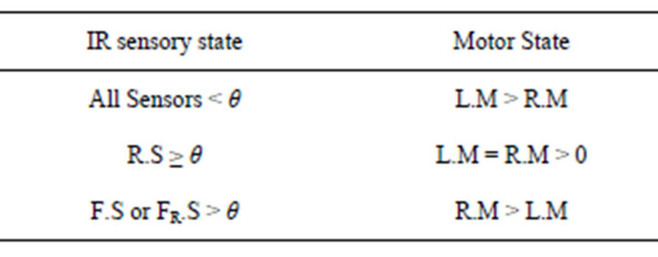
Table 1. The desired sensory-motor states for right-side wall-following behavior by SOSNN. θ is the sensor reading that keep the robot within a range ≈ 1.5 cm of the wall (θ = 500).
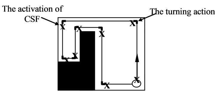
Figure 9. Robot’s right-side wall-following behavior by SOSNN controller. X represent the places where CSF were activated.
4.2.2. Second Stage (Data Abstraction & Prediction)
The main objective of this stage is to examine the validity of the second network to build the robot’s internal representation, so that, the robot can keep tracking its own relative position in the environment and to anticipate the upcoming event.
In this experiment, we left the robot, using the first network, to perform the wall-following task in the environment for 5 rounds, simultaneously with the existence of the second network whenever CSF was activated. At the beginning of each concept, the network trained both PNC and PT.
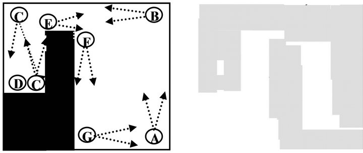
Figure 10 shows the number of concepts that the robot could identify from the environment using its camera view (A~G). From the figure we can see that our method abstracted 7 different concepts from the environment, while in [7]/[13] only 5/3 concepts were found by using the short range IR sensors, respectively. Notice that the number of concepts indicates to what degree the robot is sensitive about the environment, and as a consequence, it would results in better anticipation.
Table 2 shows the evolvement of the learning and predicting phases in the robot’s memory during the 5 complete rounds in the environment. From the table, at the first round, the robot is not able to predict neither the PNC nor PT correctly. The robot set these values randomly since it does not have experience about them. In the learning phase, however, it updates both of these values in each concept by learning online from the value of RNC and RT, respectively. It is worthwhile to mention that the robot built a suitable knowledge about the surrounding environment within the first two rounds. From the table, within the 3rd round the robot was able to predict all the PNC correctly, i.e., PNC = RNC and e decreases to 0. Although, the robot was unable to predict PT 100% correctly, i.e., PT ≠ RT, however, its value comes very close to RT and α turned out to be very close to 0.
4.2.3. Third Stage (Robot’s Internal Representation)
In [7,13], they used several slightly different environments
 (a) (b)
Figure 10. (a) The 7 concepts that robot’s camera could identify in the environment; (b) The dotted area illustrates how the robot internally represents (imagines) the whole environment.

Table 2. Second network evolvements for 5 rounds. (Each concept identified by CC’s value that automatically generated in sequential manner). RNC = the CC of the next step.
to show that their robot could capture some features from the original environment in its internal representations by monitoring the prediction error function in each step. A similar investigation was performed in this stage using environment II shown in Figure 11 (where the tunnel to the small room was closed and an extra stationary object was added to the initial environment). After the robot was trained in the original environment, i.e., its memory gained enough experience about the environment through 5 successful complete rounds, we moved the robot to environment II.
The results in Table 3 show that the robot became confused and could not predicted correctly during most of the first two rounds, i.e., PNC ≠ RNC, and the value of e increased. During the 2nd round e gradually decreaseddue to the number of changes that happened in the memory. For instance, the prediction layer of concept’s A changed from B to G, and two new branches were created in the memory to handle the new concepts, H&I and their prediction layer. From these results, we can claim that our robot, at the beginning, sensed the changes in the environment and gradually adapted its memory (see Figure 12). In round 3, all the concepts were predicted correctly.
Figure 13 shows the final memory structure after 3 rounds in environment II. From the figure we can see that due to the memory type we used, the data that referred to (environment I) was still stored in some nodes in the memory and could be recalled whenever the robot moves back to the original environment or whenever the robot faces a similar concepts in the new environment. The overall memory structure was retained with a little modification to cope with the changes in the new environment.
4.2.4. Fourth Stage (Blindfolded Navigation)
The objective of this stage is to examine the ability of the robot to replace all of its external IR sensory input with its own internal representation, i.e., repeatedly using the sequences of its own prediction for a certain number of times without external sensory input, see the dashed lines in Figure 5(b). In other words, have the robot navigate itself blindfolded in the environment.
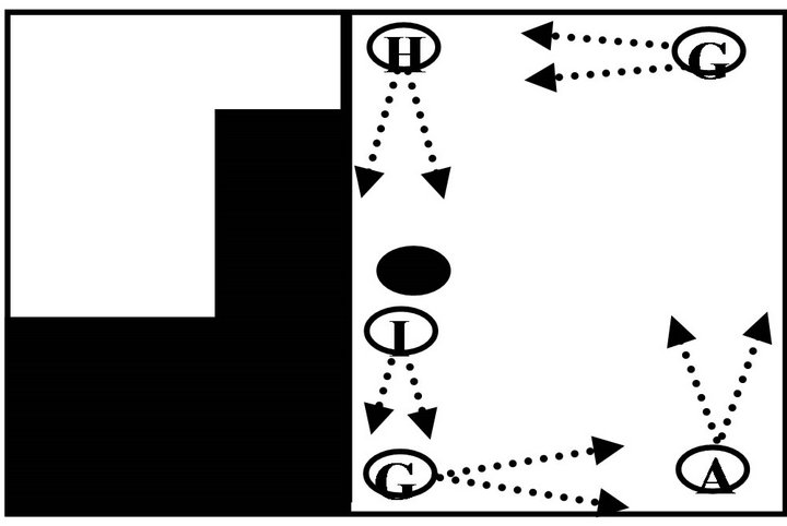
Figure 11. Environment II.


Figure 12. (e + a) during 5 rounds in environment I and 3 rounds in environment II.
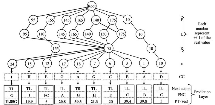
Figure 13. The final tree-type memory structure after 3 rounds in the environment of Figure 12. Thick lines illustrate the changes that occurred in the memory. The robot used some of the past experiences to predict concept in the new environment.
In this stage, after the robot trained in the original environment for 5 rounds, we removed the surrounding environment completely, eliminated the external sensory inputs, and let the robot move in a wide space using only the last found sequence of the concepts in its memory.
Figure 14 shows the robot’s best behavior. It is interesting to note that the robot built experiences about the environment in its memory sensitive enough so that it could navigate in the environment without any interacttion with the external world. All the concepts were memorized correctly, and the robot moved according to the environment’s layout. Unfortunately, the robot has slightly shifted its movement in each round, and this was probably due to the error in predicting the time of each concept a, as can be seen from Table 2.
5. Discussion and Future Work
We have presented some initial experiments with the aim to contribute toward the development of robot models in sensorimotor abstraction, simulation and anticipation. In particular, and unlike most previous related work, we have here presented: 1) a robot equipped with a video camera to extract data from the environment during its navigation, and 2) a tree-type memory structure to store this data in a simple manner as the robot experiences it to use to anticipate upcoming events and to guide its behavior in the absence of external inputs.
Our experiments show that the proposed algorithm successfully built internal representations of the environment through 7 concepts in its memory. These representations were capable of predicting upcoming concepts

Figure 14. Robot’s behavior during the navigation in a wide space using only the sequences of its internal representation for 3 rounds.
and of navigating the robot blindfolded in the environment, replacing missing IR-sensory input.
The results in the 2nd stage indicated that our algorithm had memorized the sequences of concepts found in the environment, as well as the robot’s behavior in each one. The results in the 3rd stage showed that the internal representation had captured the topology of the original environment and dynamically adapted to changes in it. The overall memory structure remained as it is and a little change occurred to cope with the changes in the environment. With such memory structure, the robot’s previous knowledge could be recalled easily. In the final stage, the robot indeed was able to navigate, to some degree, blindfolded using only its own internally built representation without any external world interaction. The robot used its “mind” to navigate from one concept to another in the environment by operating through a series of actions and situations that it learned. The robot’s memory was not very good at predicting the real time needed for each concept, but neither can humans (Figure 1(c)), and this caused a little delay in the robot’s movement, as illustrated in Figure 14.
Although some studies have reported on the issue of robot imaginations and anticipations in different ways (e.g., [21]), where the robot can use its sensorimotor representation in the brain to simulate its movement internally before the actual movement and to reason about its ability to perform the task in a short time and a safe manner, the robot, however, has been told the layout of the environment and/or the position of the targets in advance. We showed in this study, that the robot could build an environment’s map and an appropriate sequence of events in it through its own experiences. The robot can then use this data to recover any missing or corrupted data and even plan its future movement within its internal representation before any actual move (Figure 10(b)).
We believe that the work presented here illustrates some promising directions for further experimental investigations of visiomotor abstraction and for further developments of the synthetic phenomenology approach in general.
As a possible future set of experiments, it would be interesting to try to improve the learning algorithm of the second network by building a higher-level to control the prediction-layer operations in the prediction phase (experiment 2). This will decrease the learning time for newly created prediction-layers. Currently, we are trying to improve the robot’s sight sense ability to enhance the time prediction, by introducing a new 3D image processing algorithm to the system. We are also trying to improve the memory operating ability so that the robot can guess the result of an action that it has never gone through before and which is similar to a combination of actions that it has experienced earlier.
6. Acknowledgements
Supported by grants to KM from Japanese Society for Promotion of Sciences, and the University of Fukui. Authors would like to thank Mr. Edmont Katz for his valuable discussion.
REFERENCES
- M. S. Gazzaniga, “The Cognitive Neurosciences III,” MIT Press, Cambridge, 2004.
- F. J. Varela, E. Thompson and E. Rosch, “The Embodied Mind: Cognitive Science and Human Experience,” MIT Press, Cambridge, 1991.
- A. Clark and R. Grush, “Towards a Cognitive Robotics,” Adaptive Behavior, Vol. 7, No. 1, 1999, pp. 5-16. doi:10.1177/105971239900700101
- R. Grush, “The Emulation Theory of Representation: Motor Control, Imagery, and Perception,” Behavioral and Brain Sciences, Vol. 27, No. 3, 2004, pp. 377-435. doi:10.1017/S0140525X04000093
- G. Hesslow, “Conscious Thought as Simulation of Behaviour and Perception,” Trends in Cognitive Science, Vol. 6, No. 6, 2002, pp. 242-247. doi:10.1016/S1364-6613(02)01913-7
- F. Linåker and L. Niklasson, “Extraction and Inversion of Abstract Sensory Flow Representations,” Proceedings of the 6th International Conference on Simulation of Adaptive Behavior, from Animals to Animates, Vol. 6, MIT Press, Cambridge, 2000, pp. 199-208.
- J. Stening, H. Jacobsson and T. Ziemke, “Imagination and Abstraction of Sensorimotor Flow: Towards a Robot Model,” In: R. Chrisley, R. Clowes and S. Torrance, Eds., Proceedings of the Symposium on Next Generation Approaches to Machine Consciousness, Hatfield, 2005, pp. 50-58.
- J. Stening, “Exploring Internal Simulations of Perception in a Mobile Robot Using Abstractions,” Masters Thesis, School of Humanities and Informatics, University of Skövde, Sweden, 2004.
- T. Ziemke, D. A. Jirenhed and G. Hesslow, “Internal Simulation of Perception: A Minimal Neuro-Robotic Model,” Neurocoputing, Vol. 68, 2005, pp. 85-104. doi:10.1016/j.neucom.2004.12.005
- F. Linåker and L. Niklasson, “Time Series Segmentation Using an Adaptive Resource Allocating Vector Quantization Network Based on Change Detection,” Proceedings of the International Joint Conference on Neural Networks, IEEE Computer Society, Vol. 6, 24-27 July 2000, pp. 323- 328.
- D. S. Nolfi and J. Tani, “Extracting Regularities in Space and Time through a Cascade of Prediction Networks: The Case of a Mobile Robot Navigating in a Structured Environment,” Connection Science, Vol. 11, No. 2, 1999, pp. 125-148. doi:10.1080/095400999116313
- D. N. Lee and J. A. I. Thompson, “Vision in Action: The Control of Locomotion,” In: D. Ingle, M. A. Goodale and R. J. W. Mansfield, Eds., Analysis of Visual Behavior, MIT Press, Cambridge, 1982, pp. 411-433.
- G. Hesslow, “Will Neuroscience Explain Consciousness?” Journal of Theoretical Biology, Vol. 171, No. 1, 1994, pp. 29-39. doi:10.1006/jtbi.1994.1209
- D. A. Jirenhed, G. Hesslow and T. Ziemke, “Exploring Internal Simulation of Perception in Mobile Robots,” In: K. Arras, C. Balkenius, A. Baerfeldt, W. Burgard and R. Siegwart, Eds., The 4th European Workshop on Advanced Mobile Robotics, Lund University Cognitive Studies, Vol. 86, Lund, 2001, pp. 107-113.
- T. Ziemke, D. A. Jirenhed and G. Hesslow, “Blind Adaptive Behavior Based on Internal Simulation of Perception,” Department of Computer Science, University of Skövde, Sweden, 2002.
- N. Jakobi, P. Husbands and I. Harvey, “Noise and the Reality Gap: The Use of Simulation in Evolutionary Robotics,” Proceedings of the Third European Conference on Advances in Artificial Life, Lecture Notes in Computer Science, Vol. 929, Springer Verlag, London, 1995, pp. 702-720.
- T. Taylor, S. Geva and W. W. Boles, “Monocular Vision as a Range Sensor,” In: M. Mohammadian, Ed., Proceedings of International Conference on Computational Intelligence for Modeling, Control and Automation, 2004, pp. 566-575.
- S. Schaal and C. G. Atkenson, “Robot Juggling: An Implementation of Memory-Based Learning,” Control System Magazine, Vol. 14, No. 1, 1994, pp. 57-71. doi:10.1109/37.257895
- F. Alnajjar, I. MohdZin and K. Murase, “A Spiking Neural Network with Dynamic Memory for a Real Autonomous Mobile Robot in Dynamic Environment,” Proceedings of International Joint Conference on Neural Networks, Hong Kong, 1-6 June 2008, pp. 2207-2213.
- F. Alnajjar and K. Murase, “Self Organization of Spiking Neural Network that Generates Autonomous Behavior in a Real Mobile Robot,” International Journal of Neural Systems, Vol. 16, No. 4, 2006, pp. 229-239. doi:10.1142/S0129065706000640
- R. Vaughan and M. Zuluaga, “Use Your Illusion Sensorimotor Self-Simulation Allows Complex Agents to Plan with Incomplete Self-Knowledge,” Proceedings of Ninth International Conference on Simulation of Adaptive Behavior, Rome, 2006, pp. 298-309.