Journal of Information Security
Vol.08 No.04(2017), Article ID:80038,21 pages
10.4236/jis.2017.84023
Cybersecurity: Time Series Predictive Modeling of Vulnerabilities of Desktop Operating System Using Linear and Non-Linear Approach
Nawa Raj Pokhrel1, Hansapani Rodrigo2, Chris P. Tsokos1
1Department of Mathematics and Statistics, University of South Florida, Tampa, FL, USA
2School of Mathematical and Statistical Sciences, University of Rio Grande Valley, Edinburg, TX, USA

Copyright © 2017 by authors and Scientific Research Publishing Inc.
This work is licensed under the Creative Commons Attribution-NonCommercial International License (CC BY-NC 4.0).
http://creativecommons.org/licenses/by-nc/4.0/


Received: October 4, 2017; Accepted: October 28, 2017; Published: October 31, 2017
ABSTRACT
Vulnerability forecasting models help us to predict the number of vulnerabilities that may occur in the future for a given Operating System (OS). There exist few models that focus on quantifying future vulnerabilities without consideration of trend, level, seasonality and non linear components of vulnerabilities. Unlike traditional ones, we propose a vulnerability analytic prediction model based on linear and non-linear approaches via time series analysis. We have developed the models based on Auto Regressive Moving Average (ARIMA), Artificial Neural Network (ANN), and Support Vector Machine (SVM) settings. The best model which provides the minimum error rate is selected for prediction of future vulnerabilities. Utilizing time series approach, this study has developed a predictive analytic model for three popular Desktop Operating Systems, namely, Windows 7, Mac OS X, and Linux Kernel by using their reported vulnerabilities on the National Vulnerability Database (NVD). Based on these reported vulnerabilities, we predict ahead their behavior so that the OS companies can make strategic and operational decisions like secure deployment of OS, facilitate backup provisioning, disaster recovery, diversity planning, maintenance scheduling, etc. Similarly, it also helps in assessing current security risks along with estimation of resources needed for handling potential security breaches and to foresee the future releases of security patches. The proposed non-linear analytic models produce very good prediction results in comparison to linear time series models.
Keywords:
ARIMA, NVD, ANN, OS, SVM, CVE, SMAPE

1. Introduction
A computer system is a collections of hardware and software components working together to perform a well defined objective as a unified whole entity. One of the core software components of the computer system is the Operating System (OS). An OS is a resource manager or a complex interactive software system. It enables the higher level application software to communicate with its hardware and memory. Vulnerabilities always exist on such software and causes tremendous security risks to software companies, developers, and individual users. Once an attacker compromised an Operating System via any vulnerability, this implies logically the whole computer system is in control of the hacker. If the computer system itself is in control of unauthorized people, very significant consequences occur in tremendous financial loses, among other serious damages.
It is well known that the overall rates of the software vulnerabilities are extensively increasing [1] . According to the Secunia Vulnerability Review 2015, the number has increased to 55% in the past five years, and an 18% increase from 2013 to 2014 [2] . Similarly, Flexera Software reports that a 39% increase in the five year trend, and a 2% increase from 2014 to 2015 [3] . A Microsoft vulnerabilities study report in 2015 by Avecto Software Company reported that there is a significant uplift in the total number of vulnerabilities users are exposed to, rising 52% a year to year basis [4] . The documented facts and figures from the well established software institutions reveal the current increasing trend in number of software vulnerabilities that offer a significant problem to the industry. If these vulnerabilities are exploited and it is the objective of the hacker, we can realize a tremendous amount of damages and losses to software developers, government institutions, giant corporations, educational institutions, end users, and all possible stakeholders associated with this domain.
Some recent analytical study and modeling of general vulenerabilities can be found in [5] [6] [7] . It is not possible to develop an OS software free of vulnerabilities. On the contrary, we can have a precise estimation of vulnerabilities along with its trends, level, and seasonality based on the historical data. Once we have a better estimation of the number of vulnerabilities, as per our demand with respect to the calender time, it would assist us to be well prepared to manage the forthcoming risks. At the same time, we can make diversity planning such as practical contingency plans, provisioning the backup capabilities, allocation of human and financial resources effectively and efficiently to achieve our mission, to be protected from the hackers.
Figure 1, gives a schematic view of the market share of Desktop OS worldwide, with Microsoft dominating the subject industry. In broad classification in-terms of the type of OS, two Operating Systems exist in the market as described in Figure 2. A proprietary Operating System which in particularly conceptualizes, designs, and is sold by the specific company and does not share the source code to the public.
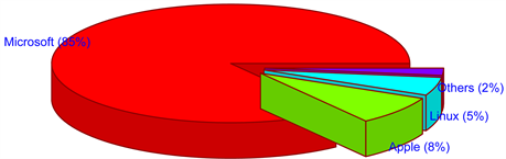
Figure 1. Market share of desktop os based on netmarketshare data.

Figure 2. Classification of desktop OS.
Microsoft and Apple are the two giant companies developing proprietary desktop Operating Systems. Similarly, Linux develops one of the non proprietary desktop Operating System referred as Linux kernel. According to Netmarketshare up to July 2016, [8] almost 85% of the market share of desktop Operating System is captured by the Microsoft company. Likewise, 8% of market share is captured by the Apple company and approximately 5% from Linux kernel which is graphically illustrated in Figure 1, above. To be more precise, out of 85% market coverage of all Microsoft’s existing operating system, Windows 7 covers almost 48%. There is only one Operating System developed by the Apple company that is Mac OS X. On the other hand Linux develops Linux kernel and is considered as one of the oldest Operating System. This OS has minimum market coverage according to Netmarketshare data. From the reported facts and popularity among the users if we aggregate the total market share of three desktop Operating System, they almost cover most of the market share in the Desktop Environment. Thus, it is appropriate to select Windows 7, Mac OS X, and Linux Kernel for our present study. These Operating Systems are the product of three industry leaders, Microsoft, Apple, and Linux.
The schematic network of Desktop Operating Systems, given by Figure 2 above, displays a layout of the process that our analytic study will follow. In the present study, we have developed analytic vulnerability forecasting models using time series analysis via linear and non-linear approaches. The developed forecasting models completely capture the complicated linear and non-linear interrelationship between past data points and extrapolate those relationship into the future. We have implemented Autoregressive Integrated Moving Average (ARIMA) to incorporate the linear behavior of the signal in conjunction with trend, level and seasonality. To capture the non-linear characteristics of the signal, we are using Artificial Neural Network (ANN) and Support Vector Machine (SVM). Finally, we have compared the final outcomes of linear and non-linear models that best fit the actual data set. Based on the outcomes of the developed models, all the stakeholders associated with Operating System will find our predictive models of significant importance. As a software developer, one can evaluate and proceed to be confident with their strategic and operational policies. They can make the appropriate plans to allocate the human and financial resources effectively and efficiently. Moreover, they can make streamline patch decisions about OS and can utilize the outcomes for security testing procedure of the Operating System. Additionally, knowing the future vulnerabilities offer several benefit; one can identify the OS that are in need to be restricted to reduce its vulnerability, the predictive vulnerability score can be used for competitive market analysis, monitor the behavior of competing OS using the forecasted vulnerability etc. But most importantly this information is extremely important to the IT manager for his/her strategic planning to minimize the risk of chosen OS that will not be exploited. Finally, our results offer a unique marketing strategy for purchasing the best OS available in the market place that will have the best (smallest) future vulnerabilities.
In the present research our objective is to develop a high quality analytical forecasting model utilizing both linear and nonlinear methods to predict the number of vulnerabilities of a given operating system. In addition we will perform statistical evaluations of other models that perform the same task the predicting process of OS. The selected model provides overall trend and behaviour of the OS ahead of time; OS companies can make strategical and operational decisions such as secure deployment of OS, facilitate backup provisioning, disaster recovery, diversity planning, and maintenance scheduling. Similarly, all the stakeholders related to the OS can access the current sercurity risk along with estimation of resources needed for handling potential security breaches and for see the future releases of security patches. Finally, the predictive results can be used for the competitive analysis of the product which significantly helps to develop the marketing strategies for the respective OS.
Our research paper is organized as follows: Section 2 introduces and explains the literature review. Section 3 explores the datasets and explanation of major methods employed in our study. In Section 4, the core analysis and predictive power of the developed models are discussed. Finally, the usefulness of our analytical model is presented along with our future research goals.
2. Related Research
During the past years, scientists and researchers have given tremendous amounts of time and effort to develop vulnerability forecasting models to predict the future vulnerabilities of OS taking into consideration of their historical behavior with reported data. One can characterize these proposed developed models into two categories.
1) Code Characteristics Based Models: These types of models are relying on finding out the relationship between attributes of the code with its corresponding vulnerabilities. Rahimi and Zargham, [9] proposed a vulnerability scrying approach, that is, a vulnerability discovery prediction method based on code properties and quality. S. Riccardo et al. [10] proposed a machine learning approach to predict which components of the software applications contain security vulnerabilities using a text mining approach. This approach identified a series of vulnerable terms contained in its source code and was used to compute its frequency. Based on the frequency, they proceeded to forecast its future. Shin et al. [11] performed an empirical study with traditional metrics of complexity, code churn, and faulty history using a large open source project to determine whether fault prediction models can be used for vulnerability prediction models. Nguyen and Tran, [12] proposed a component dependency graph to predict vulnerable components using machine learning methodology. All the mentioned approaches requires source code to built the models, source code of the OS is dynamic in nature and it is not available to public in case of proprietary OS.
2) Statistical Density Based Models: In this category, vulnerability forecasting models are based on historical data of the Operating System. To fulfill this objective, various kinds of models have been developed, mainly Alhazmi-Malaiya Logistic (AML) with different versions, [13] Poissons Log Arithmetic Model, [14] , Rescorals Exponential Models [15] , and Andresons Thermoodynamics Model [16] . All the developed models are based on their underlying assumptions and defined framework and none of them considers the non linear behavior of the signal.
For code characteristics based models, we need a source code of the given software to develop statistical models. In reality, source code of the commercial OS is not available to the public. Each and every day new vulnerability comes into existence and we need to handle new vulnerabilities, thus the software should be continuously updated which implies that the source code changes with respect to the life cycle of the software. A company always updates its software so as to fulfill the demands of current or potential customers and hence we need to update the source code regularly. Thus, process of making source code is always dynamic in nature. One of the prominent question that arises here is “how can we forecast the future vulnerabilities by utilizing static source code?”. Knowing very well that no OS is with zero or no vulnerability at all and this will continue in the future. On the other hand, considering statistic density based models, that have been developed are based on a series of underlying assumptions and criteria that may or may not be applicable. For instance, Rescola Linear Model (RL) attempts to fit vulnerability finding rates linearly with time but in reality situations are different for nonlinear behaviours. Because of such limitations that exist on both categories, we should identify an alternative approach to forecast the future vulnerability of an OS by using time series analysis. Our model considers trend, level, and seasonality components if they exist. Similarly, to analyze the non-linear behavior of the number of vulnerabilities, we implemented ANN and SVM methodology.
3. Data and Methodology
We have directly extracted the vulnerability data from the National Vulnerability Database (NVD). It is the U.S. governments repository that integrates publicly available vulnerability resources and provides the common references to the industry resources. NVD is a product of the National Institute of Standards and Technology (NIST), Computer Security Division and is sponsored by the Department of Homeland Security’s National Cyber Security Division. It contains reported vulnerabilities based on their Common Vulnerabilities and Exposures (CVE) identifier. The total number of vulnerabilities with respect to time in monthly basis is the fundamental quantitative values for our analysis and modeling. The schematic diagram in Figure 3 describes the holistic idea about the datasets and methods employed in our study.
We have collected the vulnerabilities for each Operating System, the earliest available data from NVD to December 2015 as training data, however, the whole
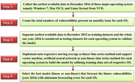
Figure 3. Bird’s eye view of data collection and method selection via flow chart.
one year, 2016 data is considered as testing data to validate our model. We summed the total vulnerabilities over a monthly period. Linear and non-linear time series methods are implemented to select the best model with minimum forecasting error for each OS.
The following Table 1, shows the summary of descriptive analysis of the training data. It includes the total number of vulnerabilities on monthly basis, collection period, and monthly average. From the table below, we can conclude that average number of vulnerabilities was highest in Mac OS X followed by Linux kernel and Windows 7.
Our analysis begins by investigating the total number of vulnerabilities accumulated by month for three OS, Figure 4, below reveals the overall variation in total number of vulnerabilities of Mac OS X.
Inspecting Figure 4, the trend of the number of vulnerabilities of MAC OS X Operating System, it is clearly visible that initially the number of vulnerabilities are low and fairly stable, as a function of time. There is a high spike at the end of year 2015. In 2015 the number of vulnerabilities is almost four times greater

Table 1. Descriptive statistics of vulnerability datasets: mac os x, windows 7, and linux kernel os.
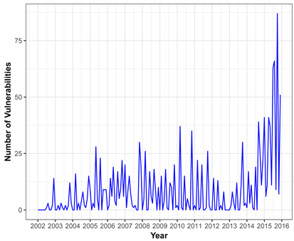
Figure 4. Time series pattern of mac os x.
than in previous years. One of the prominent reasons is due to the rapid market share gains of Mac OS X which leads to growing attack surface for sensitive data. There are several malicious malware introduced in 2015, for instance, XcodeGhost which inserts malicious components in to the applications made with Xcode [17] (Apple’s official tool for developing IOS and OS Apps).
Figure 5, shows the overall trend of the number of vulnerabilities of Windows 7 OS having a very nonlinear behavior. Initially number of vulnerabilities seems low but after a short period of time, we can see a significance increase and decrease of the number of vulnerabilities as a function of time. There is a very sharp increase in the number of vulnerabilities in 2012, 2014 and 2015 for windows 7. “Secunia Vulnerability Review 2014”, reported that the majority of the vulnerabilities on Windows 7 come from the non-Microsoft software like Google Chrome, Adobe Flash Player and others rather than the major defect in OS itself.
To incorporate the sharp random fluctuations of the number of vulnerabilities in each year, we initially believe that non linear time series methods are the suitable method to build the analytical forecasting model. If the IT manager had a good forecast of the large number of vulnerabilities, the subject of our study, he/she would have taken appropriate action to address this critical issue.
The overall trend of the number of vulnerabilities of Linux Kernel OS is demonstrated by Figure 6 from 2001 to 2015. Even though there is an increasing and decreasing trend, it would be fair to say that there is a significant variation in the number of vulnerabilities especially in 2014 and 2015, with more than
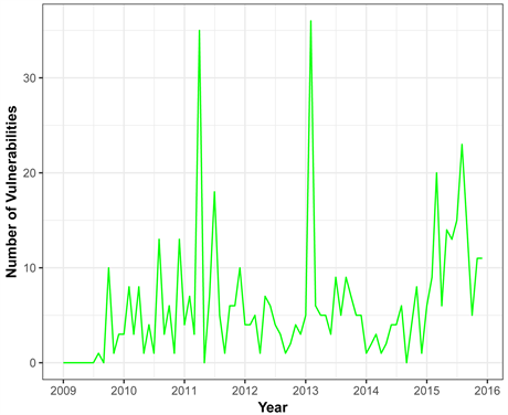
Figure 5. Time series pattern of windows 7 os.
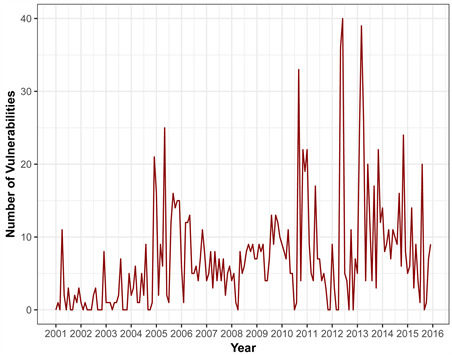
Figure 6. Time series pattern of linux kernel os.
double the number of vulnerabilities for the previous year. Years 2014 and 2015 were difficult years for Linux OS in terms of security perspective, for example “Heartbleed” is the severe vulnerability detected in OpenSSL that left large number of cryptographic keys and private data from important sites and services in the Internet that were open to the hackers. Similarly, Shellshock is the vulnerability that is dominantly used in Linux OS command line Shell, also called Bash or GNU Bourne Again Shell left the door open for a hacker to lunch malicious attack.
All three graphs mentioned above, Figures 4-6, provides a pictorial view comparison of the number of vulnerabilities of the three OS, MAC OS X, Windows 7 OS, and Linux Kernel OS from respective calender time, on monthly basis. It does not seem obvious seasonality components exist but random fluctuations have a significant influence on each case. It is clear that each of the OS has some sort of increasing or decreasing trend for a specific period of time and all of sudden some spikes come and changes the behavior of the signal. To incorporate all the mentioned facts, we have employed linear and non linear techniques to build the best analytic forecasting model. The following section provides a brief explanation of the techniques employed in this study.
3.1. Autoregressive Integrated Moving Average Process (ARIMA) Model
Autoregressive Integrated Moving Average (ARIMA) models, are commonly used for linear models for univariate time series analysis. To construct the ARIMA model to forecast the vulnerabilities requires three steps. Before going to the first step, it is necessary to check if the vulnerability data is stationary, this implies that the number of vulnerabilities associated with each operating system shows no trend over monthly observations. We have implemented Dicky-Fuller and Philips-Perron [18] unit root test to examine the stationarity of the ARIMA models. Whenever stationarity of the ARIMA models is established, the first steps to build the ARIMA model requires to identify the appropriate structure and order of the model. The ARIMA model includes autoregressive terms (AR), moving average terms (MA), and differencing operations. An ARIMA model structure is represented by (p, d, q) where p is AR process, d is number of differences (filtering) and q is MA process. An AR(n) specifies number of immediately preceding vulnerabilities in the series that are used to forecast vulnerabilities at present. For example, AR(1) means the number of vulnerabilities at time t = 1 rely on the numbers of vulnerabilities at t − 1. Differencing term d is the degree of differencing (the number of times the vulnerability data have had past value subtracted) required to achieve the stationarity condition of the process. The MA(n) shows that present vulnerabilities have a relationship with past vulnerabilities, white noise error terms or random shocks. The random shocks are assumed to be independent and come from the same probability distribution. For example, MA(1), AR(1) means that the number of vulnerabilities at time t = 1 relies on numbers of past prediction errors at t − 1. The general equation of the model ARIMA(p, d, q) is given by:
(1)
where,
= differenced in series
c = a constant
=coefficients or weights
p = order of the AR term
q = order of MA term
= residuals at time t
The second step is to construct the ARIMA model is to identify the number of parameters that are necessary to be included in the model which is a function of the order of the model. Furthermore we need to obtain estimates of the parameter that drive the model. We have implemented a graphical and statistical approach to find out the parameters used to forecast the vulnerabilities. For the graphical method, autocorrelation function (ACF) and partial autocorrelation function (PACF) is implemented. On the other hand, estimation of the required parameters requires complicated iteration procedure using maximum likelihood or non linear least square estimation methods. The final step of ARIMA is a diagnostic checking and forecasting vulnerabilities of the OS. The complete model fitting process is based on the law of principle of parsimony where the best possible model is the simplest with respect to accurately forecast the vulnerability of a given OS.
Utilizing the model building procedure of ARIMA model namely model formulation, model estimation, and model checking or model verification, we have developed three models for Mac OS X, Windows 7, and Linux as shown by the following Equations (2), (3), and (4) respectively:
Mac OS X (ARIMA(1,1,3)):
(2)
Windows 7 (ARIMA(2,1,1)):
(3)
Linux Kernel (ARIMA(2,0,3)):
(4)
3.2. Artificial Neural Network (ANN)
Artificial Neural Networks (ANN) is one of the useful and popular method, which have been used in forecasting using time series data. A wide variety of applications can be found in market predictions, meteorological and network traffic forecasting [19] [20] [21] [22] , where most of them have used feed-forward ANN models in a sliding window format over the input sequence. The major advantage of neural networks is that they are data driven and does not require restrictive assumptions about the form of the basic model. Any feed forward ANN model consists of three or more layers called input, hidden, and output. The operational structure of the ANN model for the subject study are demonstrated below by Figure 7, and the final outcome of the ANN with one hidden node would be expressed analytically by:
(5)
where is the total number of vulnerabilities reported in month t, p is the number of lags (number of vulnerabilities reported in the past p months) and the H is the number of hidden nodes, g and f are the activation functions
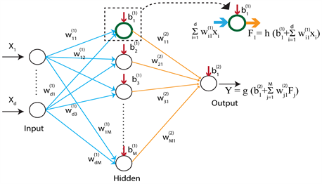
Figure 7. The architecture of the ann model used for os.
associated with the hidden and the output nodes. In order to have a better generalization with the ANN model, we need to develop new procedures. Here, in our analysis, we have used different number of lags and select the model with minimum Mean Absolute Error. In addition to that we have used time series cross validation (forecast evaluation with a rolling origin) methods to identify the optimal number of hidden nodes, which refelects on the quality of the forecast of a given OS.
Figure 7, shows the basic architecture of an ANN and it represents a multivariate non-linear function mapping between a set of inputs and outputs variables (Bishop, 1995). These networks are organized as several interconnected layers. Each layer is a collection of artificial neurons (nodes) where the connections are governed by the corresponding weights. Data have been fed through the input layer, and then they pass through the one or more hidden layers, and the final outcome is given by the output layer.
One of the challenges that we face when we use ANN in time series prediction in identifying the number of inputs which is not fixed. We used a procedure to identify the best possible number of lags.
3.3. Support Vector Machine (SVM)
Traditionally SVMs are used for classification in pattern recognition applications. These learning algorithms have also been applied to general regression analysis, the estimation of a function by fitting a curve to a set of data points. The application of SVMs to general regression analysis case is called Support Vector Regression (SVR) and is vital for many of the time series prediction applications. SVMs used for time series prediction span many practical application areas from financial market prediction to electric utility load forecasting to medical and other scientific fields. One of the advantage in SVM is that it just correspond to a convex optimization problem when determining the model parameters and hence easily can be implemented. In using Support Vector (SV) regression, our goal is to find a function that has at most deviation from the actually obtained targets for all the training data, and will not accept any deviation larger than that. Anything beyond the specified -will be penalized in proportion to C, which is the regularization parameter. This can be explained with a linear function of the form
(6)
where our goal is to minimize
(7)
with respect to the constraints
(8)
The constant , determines the trade-off between the flatness off and the amount up to which deviations larger than are tolerated. Support vector machine can be generalized to deal with a nolinear function , and minimize the weights with respect to the constraint
(9)
such that , and where, are the Lagrange multipliers, Q is a l by l positive semidefinite matrix with, and is the kernel. However, in SVR we have no control on how many data vectors from the dataset become support vectors and the correct choice of kernel parameters is crucial for obtaining desirable results [23] . Our objective is to conduct extensive analytical driven search procedure on the parameter space to obtain the optimal set of parameters that drive the model.
3.4. Analysis with ANN and є SV Regression
We began our analysis by dividing the vulnerability dataset into two groups; Training and Testing. The testing data set consists of vulnerabilities reported in year 2016. We then normalized the data by applying the min-max normalization method. Our analysis with ANN and SV regression makes the assumption that the number of future vulnerabilities depends on the vulnerabilities identified in the present and past months (lags). The number of significant lags in the partial auto correlation function has been used initially to determine the optimal number of lags. We proceeded by carring out further analysis by changing the number of lags from 2 to 10.
The radial basis functional kernel is used to develop the SV regression models with fine-tuning the two set of parameters; gamma and the regularization parameter C. In developing the ANN model we used 10-fold cross validation method for time series. When using this techniques we incremented the training sets data, gradually shifting the training data set window one by one. This was repeated for different number of hidden nodes. The optimal analytical model is selected based on the average mean absolute error (MAE). Finally, the selected analytical model is used to make the prediction in the testing data set.
4. Analysis
Our statistical analysis follows the process that we have introduced in Section 3, where we described the overall time series trend of each OS. We need further investigation on each signal to see if any trend, cycles, and seasonality exists. Usually time series data consist of a specific trend, cycles, and seasonality. To identify the best analytical forecasting model, we will first proceed to identify the time series pattern in the data, and then select an appropriate method that will capture the patterns effectively. Figure 8 is structured in two columns; which consist of six individual graphs. In Figure 8, Figure 8(a), Figure 8(c), and
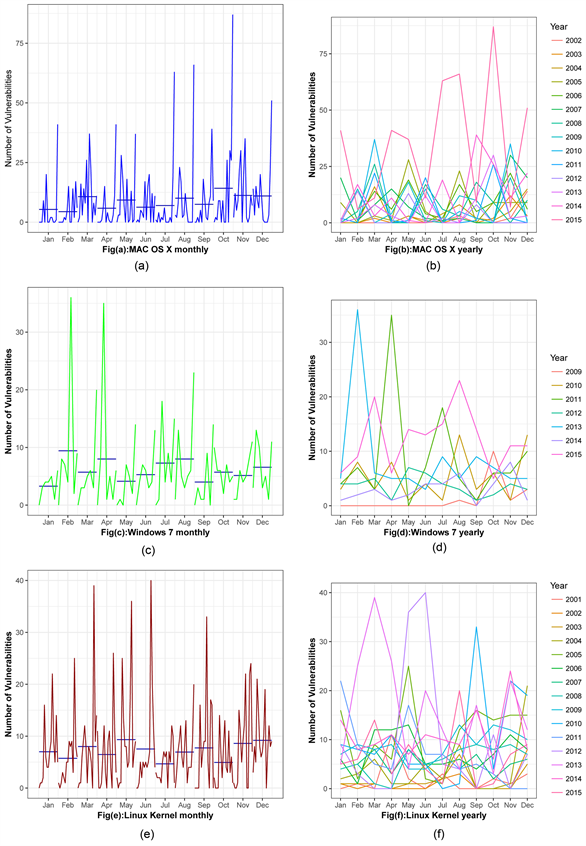
Figure 8. (a): Overall monthly deviation of mac os x os. (b): Overall yearly pattern of mac os x os. (c): Overall monthly deviation of windows 7 os. (d): Overall yearly pattern of windows 7 os. (e): Overall monthly deviation of linux kernel os. (f): Overall yearly pattern of linux kernel os.
Figure 8(e) descriebes the monthly behaviour of Mac OS X, Windows 7, and Linux Kernel OS respectively. These sub-series plots are inspected as a preliminary screening tool, that allow us for a visual inferences to be drawn from the data before proceeding to modeling and forecasting.
In Figure 8 first columns’ sub-series plots emphasize monthly patterns where the data for each month is collected together in separate mini time plots. The horizontal lines indicate the means for each month. This plot helps to find the monthly pattern over time. In each plot, none of the graph specifically are revealing any seasonal and cyclical pattern. Likewise there is not a significant variation in the means for each month.
Figure 8, confirms that there is no seasonal and cyclical pattern present on any of the OS monthly basis. We need to identify weather any seasonality or cyclic pattern exist over the year. We proceeded to plot the vulnerability data against individual “year” in which the data was observed. Figure 8, Figure 8(b), Figure 8(d), and Figure 8(f) illustrate the yearly pattern of the vulnerability of Mac OS X, Windows 7, and Linux Kernel OS respectively.
In Figure 8, Figure 8(b) shows no seasonality or cyclic behavior is present over a year. It is clearly visible that there is sharp increase of vulnerabilities in year 2015 in comparison to the other year, 2002 to 2014. However, the Mac OS X system shows a significant random variation of the number of vulnerabilities. Similiarly, in Figure 8(d) each individual year shows random fluctuations of the number of vulnerabilities over a twelve month period. We also concluded that there is no specific pattern of the behavior of the signals on a yearly basis of Windows 7 OS. Year 2009 and 2013 show the largest number of vulnerabilities followed by a significant reduction for year 2015 by a factor of 10. Lastly, Figure 8(f), the signal of each individual year shows random variation of a number of vulnerabilities for a twelve month period. Year 2010, and 2013 show the largest number of vulnerabilities followed by a significant reduction for year 2010.
We plotted vulnerabilities against the individual months in which data are observed. Similarly, plots have been developed where data from each month is overlapped. These graphs allow us to make a decision that there is no specific seasonal or cyclical pattern seen in terms of monthly or yearly basis. We have found there is a large jump of vulnerability in specific years. The remaining years exhibit fluctuations on the number of vulnerabilities but no obvious seasonal or cyclic patterns. Inspecting the signal of the number of venerability in each OS, we have found that trend, level and random fluctuations are the major ingredients to build the forecasting model. Incorporating these facts, we have utilized ANN, SVM, and ARIMA models to forecast the future level of vulnerabilities for the three OS.
Predictive Capability of Models
One of the most important criteria for evaluating forecasting accuracy is to evaluate the error (residuals) generated by the testing data sets. An optimal model is selected based on how accurately it forecast our testing data sets. We have computed Root Mean Square Error (RMSE), Mean Absolute Error (MAE), and Symmetric Mean Absolute Percentage Error(SMAPE), for each model to assist in the selection process of the best model. For each forecast error estimation lower values are preferred.
Prediction accuracy of the analytic model is one of the most important criteria to evaluate the model performance and reliability. In addition to RMSE and MAE, we utilized an error analysis based on Symmetric Mean Absolute Percent Error (SMAPE) rather than Mean Absolute Percent Error (MAPE) to convinence the validity of our model. Even though SAMPE is based on MAPE, it does consider data containing zeros and non zero values that may skew the error rate. It consist of 0% of lower bound and 200% of upper bound, thus it reduces the impact of zeros and non zero values on our data sets. The error is computed based on the analytical form defined by the equation below:
(10)
where, N is the total number of prediction intervals, is the predicted number of vulnerabilities, and is the actual number of vulnerabilities. Once we employed ANN, SVM and ARIMA model on our testing data set following optimal model are selected based on our error measurement criteria in Table 2.
Our ANN model evaluation results were quite good despite the fact that we did not have enough data to improve the training of our model. However, we believe that as more information of the subject matter becomes available the ANN model will be easier to implement and with higher accuracy in predicting the number of vulnerabilities of the present OS in the market place. For Windows 7 and Linux kernel is the analytical model, SVM driven by the final Equation (9). With reference to the Table 2, the best models are selected for each OS based on the low error rate and the law of parsimony are listed in Table 3.
From Table 3 ARIMA(1,1,3) with drift, SVM with lag 5, and SVM with lag 5 models are selected for Mac OS X OS, Windows 7 OS, and Linux Kernel OS respectively. To be more specific, the forecasting model for Windows 7 OS had the lowest SMAPE of (12.45%) which implies it is a good forecasting model. The developed model provides good fit to the vulnerability data for Mac OS X and
Table 2. Output measurement criteria on testing data sets for each os.
Table 3. List of best model selected for each os.
Linux Kernel but prediction accuracy is varied. In terms of forecasting, Linux kernel has a convincing SMAPE of (14.1%) but MAC OS X is reasonably accurate with a SMAPE (31.25%). One possible reason for high percentage error may be due to missing components in our analysis such as OS development process, patch cycles, difference in security enforcement criteria, as well as market share and popularity of the OS.
After the selection of the best model with minimum error rate, our study revealed the fact that the developed model provides a good fit for the OS datasets and can be used to forecast the future vulnerabilities. Fitting time series models to the vulnerability database is demonstrated via the graph as shown below.
Figure 9 shows the original vulnerability plot against fitted vulnerabilities of MAC OS X Operating System. Even though having random fluctuations that is increasing and decreasing behavior present in each year, our model accurately captures the holistic attributes of the signal with reasonable accuracy.
Figure 10, demonstrates results of fitted time series model and the actual vulnerabilities of the Windows 7 OS. Eventhough Windows 7 OS have limited amount of data comparing to other OS, it has lowest approximately 12% prediction error which attends to the high qualitiy of forecasting future vulnerabilities.
Figure 11 shows the fitting time series of the SVM model and the actual vulnerability data of Linux Kernel OS. Graphically our model shows a perfect fit with a prediction accuracy of 14% little bit higher than Windows 7 OS. This is probably due to very sharp increase of vulnerabilities in 2014 and a sudden decrease of in 2015.
All of the above plots 9, 10, and 11 a good fit for each OS but different degrees of prediction accuracy. From a careful reading of the fitted plots, we can conclude that best fitted model may not produce the best forecasting accuracy and vice versa. In case of Mac OS X, forecasted vulnerabilities is not that much better to the fit of data. Unlike Mac OS X, windows 7 has quite good fit but forecasted vulnerabilities are a way better than Mac OS X. We eventually used our models to forecast the future vulnerabilities of these OS and recommended choice for predicting monthly vulnerabilities is summarized by Table 4. As an example, the following Table 4 highlights the fore-casted values for the 12 months of the year 2016. From the table we can say that predicted number of vulnerabilities for 2016 for Mac OS X is highest followed by Linux kernel and Windows 7.
Initially, we split our data sets in terms of training and testing data sets. The
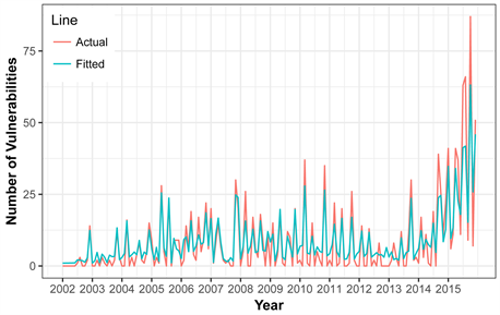
Figure 9. Original vulnerability vs. fitted vulnerabilities for mac os x os.

Figure 10. Original vulnerability vs. fitted vulnerabilities for windows 7 os.
collection period of training data set of each OS is mentioned in Table 1. Similarly, 2016 is considered as testing data sets to validate our model for all OS. Utilizing our best developed model, we forecasted 2016 vulnerabilities which are given in Table 5. Now the following Table 5 compares the total true vulnerabilities and forecasted vulnerabilities for each OS. This comparison table shows the accuracy and reliability of our developed analytical models.
Our study revealed the fact that seasonality and trends are not the major
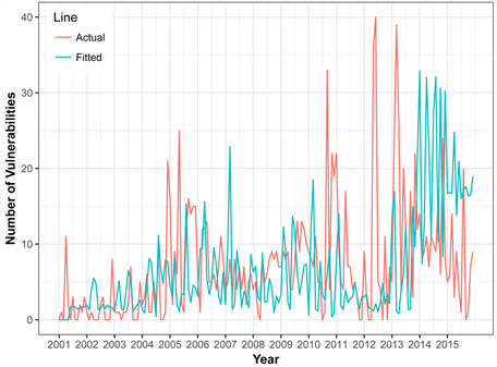
Figure 11. Original vulnerability vs. fitted vulnerabilities for linux kernel os.
Table 4. Forecasted vulnerabilities of mac os x, windows 7, and linux kernel os.
Table 5. Actual and forecasted vulnerability comparison of the os.
components of the forecasting models. Nevertheless, the level of the time series is only the significant component to build the model. This suggests that it is difficult to predict vulnerabilities based on monthly seasonal patterns or trends. Further investigation is needed whether weekly, quarterly, or annual patterns might produce remarkable trends or seasonal components but such data is not publically availiable to improve the quality of the model.
The ANN model did not perform well in forecasting the vulnerabilities because we did not have enough data to improve the training process so as to improve its forecasting accuracy. With more vulnerability data we believe that the ANN model will be very competitive in forecasting vulnerabilities of the OS.
5. Conclusions
We have developed effective linear and non linear analytic models to forecast future vulnerabilities by utilizing the vulnerability datasets of three major OS namely, Windows 7, Linux Kernel, and Mac OS X. We have not found any influential trend and seasonality components from the time series data. The proposed forecasting models reveal the fact that non linear time series models predict quite well with minimum level of error rate. The developed models can be used by the developers, the user community, and individual organization to predict the vulnerability level of their OS. Developers can examine the OS readiness by predicting the future vulnerability trend. Based on the projected vulnerabilities, they can allocate the security maintenance resources to detect the upcoming vulnerabilities. At the same time, they can implement the proper software security patch plan. The users can obtain useful information to compare different OS in terms of the risk associated with their vulnerability. They also can access the risk before patches are applied. Similarly, every organization has their own customized security policies that requires allocation of time and resources. The predictive vulnerability models we have developed can be used to quantitatively guide such policies.
Finally, the developed forecasting models of the three OS that dominate the global market can be used to predict their future vulenerabilities. The predictive vulnerabilities can be used to identify the risks associated with the forecast for each of the three OS. IT manager can implement the forecasting vulnerabilities in their operating strategies and contingency plans. Based on their predictions, each of the three manufacturing companies can make one of the decision: they are willing to live with it, make minor research and development design or major modifications. The predictive results can be used for competitive analysis of the three OS companies that are essential to their marketing strategies.
Cite this paper
Pokhrel, N.R., Rodrigo, H. and Tsokos, C.P. (2017) Cybersecurity: Time Series Predictive Modeling of Vulnerabilities of Desktop Operating System Using Linear and Non-Linear Approach. Journal of Information Security, 8, 362-382. https://doi.org/10.4236/jis.2017.84023
References
- 1. National Institute of Standard and Technology (NIST) Report 2014. http://www.nist.gov/
- 2. Secunia Vulnerability Review (2015). https://secunia.com/?action=fetch&filename=secunia_vulnerability_review_2015_pdf.pdf
- 3. Vulnerability Review (2016). http://www.flexerasoftware.com/enterprise/resources/research/vulnerability-review/
- 4. 2015 Microsoft Vulnerabilities Study: Mitigating Risk by Removing User Privileges. http://learn.avecto.com/2015-microsoft-vulnerabilities-report
- 5. Pokhrel, N.R. and Tsokos, C.P. (2017) Cybersecurity: A Stochastic Predictive Model to Determine Overall Network Security Risk using Markovian Process. Journal of Information Security, 8, 91-105. https://doi.org/10.4236/jis.2017.82007
- 6. Rajasooriya, S.M., Tsokos, C.P. and Kaluarachchi, P.K. (2017) Cyber Security: Nonlinear Stochastic Models for Predicting the Exploitability. Journal of Information Security, 8, 125-140. https://doi.org/10.4236/jis.2017.82009
- 7. Othmane, L.B., Chehrazi, G., Bodden, E., Tsalovski, P. and Brucker, A.D. (2017) Time for Addressing Software Security Issues: Prediction Models and Impacting Factors. Data Science and Engineering, 2, 107-124. https://doi.org/10.1007/s41019-016-0019-8
- 8. Desktop Operating System Market Share. https://www.netmarketshare.com/
- 9. Rahimi, S. and Zargham, M. (2013) Vulnerability Scrying Method for Software Vulnerability Discovery Prediction without a Vulnerability Database. IEEE Transactions on Reliability, 62, 395-407. https://doi.org/10.1109/TR.2013.2257052
- 10. Scandariato, R., Walden, J., Hovsepyan, A. and Joosen, W. (2014) Predicting Vulnerable Software Components via Text Mining. IEEE Transactions on Software Engineering, 40, 993-1006. https://doi.org/10.1109/TSE.2014.2340398
- 11. Shin, Y. and Williams, L. (2013) Can Traditional Fault Prediction Models Be Used for Vulnerability Prediction? Empirical Software Engineering, 18, 25-59. https://doi.org/10.1007/s10664-011-9190-8
- 12. Nguyen, V.H. and Tran, L.M.S. (2010) Predicting Vulnerable Software Components with Dependency Graphs. Proceedings of the 6th International Workshop on Security Measurements and Metrics, ACM. https://doi.org/10.1145/1853919.1853923
- 13. Alhazmi, O.H. and Malaiya, Y.K. (2006) Prediction Capabilities of Vulnerability Discovery Models. Reliability and Maintainability Symposium, 86-91. https://doi.org/10.1109/RAMS.2006.1677355
- 14. Musa, J.D. and Okumoto, K. (1984) A Logarithmic Poisson Execution Time Model for Software Reliability Measurement. Proceedings of the 7th International Conference on Software Engineering, 230-238.
- 15. Rescorla, E. (2005) Is Finding Security Holes a Good Idea? IEEE Security & Privacy, 3, 14-19. https://doi.org/10.1109/MSP.2005.17
- 16. Anderson, R. (2002) Security in Open versus Closed Systems the Dance of Boltzmann, Coase and Moore. Technical Report, Cambridge University.
- 17. https://assets.documentcloud.org/documents/2459197/bit9-carbon-black-threat-research-report-2015.pdf
- 18. Phillips, P.C. and Perron, P. (1998) Testing for a Unit Root in Time Series Regression. Biometrika, 2, 335-346.
- 19. Frank, R.J., Davey, N. and Hunt, S.P. (2001) Time Series Prediction and Neural Networks. Journal of Intelligent & Robotic Systems, 31, 91-103. https://uhra.herts.ac.uk/bitstream/handle/2299/593/102081.pdf?sequence=1
- 20. Edwards, T., ansley, D., Frank, R. and Davey, N. (1997) Traffic Trends Analysis using Neural Networks. Procs of the Int Workshop on Applications of Neural Networks to Telecommunications. http://hdl.handle.net/2299/7171
- 21. Patterson, D.W., Chan, K.H. and Tan, C.M. (1993) Time Series Forecasting with Neural Nets: A Comparative Study. Procs the International Conference on Neural Network Applications to Signal Processing, 269-274.
- 22. Bengio, S., Fessant, F. and Collobert, D. (1995) A Connectionist System for Medium-Term Horizon Time Series Prediction. Proc. Intl. Workshop Application Neural Networks to Telecoms, 308-315.
- 23. Cortes, C. and Vapnik, V. (1995) Support-Vector Networks. Machine Learning, 20, 273-297. https://doi.org/10.1007/BF00994018