Journal of Modern Physics
Vol.4 No.12(2013), Article ID:40913,8 pages DOI:10.4236/jmp.2013.412195
Critical Line Back-Bending Induced either by Finite Nc Corrections or by a Repulsive Vector Channel
1Departamento de Física, Universidade Federal de Santa Catarina, Florianópolis, Brazil
2Departamento de Física, Fundação Universidade Regional de Blumenau, Blumenau, Brazil
Email: r.denke@posgrad.ufsc.br, marcus@fsc.ufsc.br
Copyright © 2013 Robson Z. Denke et al. This is an open access article distributed under the Creative Commons Attribution License, which permits unrestricted use, distribution, and reproduction in any medium, provided the original work is properly cited.
Received August 28, 2013; revised September 29, 2013; accepted October 26, 2013
Keywords: QCD Phase Diagram; NJL Model
ABSTRACT
We analyze the two flavor version of the Nambu-Jona-Lasinio model with a repulsive vector coupling , at finite temperature and quark chemical potential, in the strong scalar coupling
  regime. Considering GV = 0, we review how finite Nc effects are introduced by means of the Optimized Perturbation Theory (OPT) which adds a
  term to the thermodynamical potential. This
  suppressed term is similar to the
  contribution obtained at the large-Nc limit when GV ≠ 0. Then, scanning over the quark current mass values, we compare these two different model approximations showing that both predict the appearance of two critical points when chiral symmetry is weakly broken. By mapping the first order transition region in the chemical potential-current mass plane, we show that, for low chemical potential values, the first order region shrinks as μ increases but the behavior gets reversed at higher values leading to the back-bending of the critical line. This result, which could help to conciliate some lattice results with model predictions, shows the important role played by finite Nc corrections which are neglected in the majority of the works devoted to the determination of the QCD phase diagram. Recently the OPT, with GV = 0, and the large-Nc approximation, with GV ≠ 0, were compared at zero temperature and finite density for one quark flavor only. The present work extends this comparison to finite temperatures, and two quark flavors, supporting the result that the OPT finite Nc contributions naturally mimic the effects produced by a repulsive vector interaction.
1. Introduction
Although most of the results obtained up to now seem to support the quantum chromodynamics (QCD) critical point (CP), an interesting observation against its existence comes from the numerical simulations of QCD at imaginary chemical potential by de Forcrand and Philipsen [1-3] which shows that the region of quark masses (mc) where the transition is presumably of the first order (for quark masses smaller than the physical ones), tends to shrink for small positive values of the chemical potential as shown in the upper panel of Figure 1. Conversely, according to models supporting the critical point, the first order region should expand when the chemical potential increases, so that the physical quark mass point hits the critical line at some finite value of the temperature and chemical potential as shown in the bottom panel of Figure 1. A possible explanation for the disagreement between the “exotic” scenario (Figure 1, upper panel) and the “standard” scenario (Figure 1, bottom panel) has been given in [4,5] where it was suggested that a strong (repulsive) vector coupling may account for the initial shrinkage of the first order region, that would then start expanding again at larger values of the chemical potential leading to the back-bending of the critical surface and the recovery to the CP at the physical quark mass values. As a result, two critical points should appear for a given range of (small) quark masses, as argued by Bowman and Kapusta [6] who investigated the Linear Sigma Model (LSM) including thermal fluctuations and considered small values for the pion mass. A pictorial view of this peculiar situation is given by Figure 2 which illustrates a possible back-bending scenario in the two-flavor case. In the more traditional T − μ plane, these two critical points are located at the end of two first order transi-
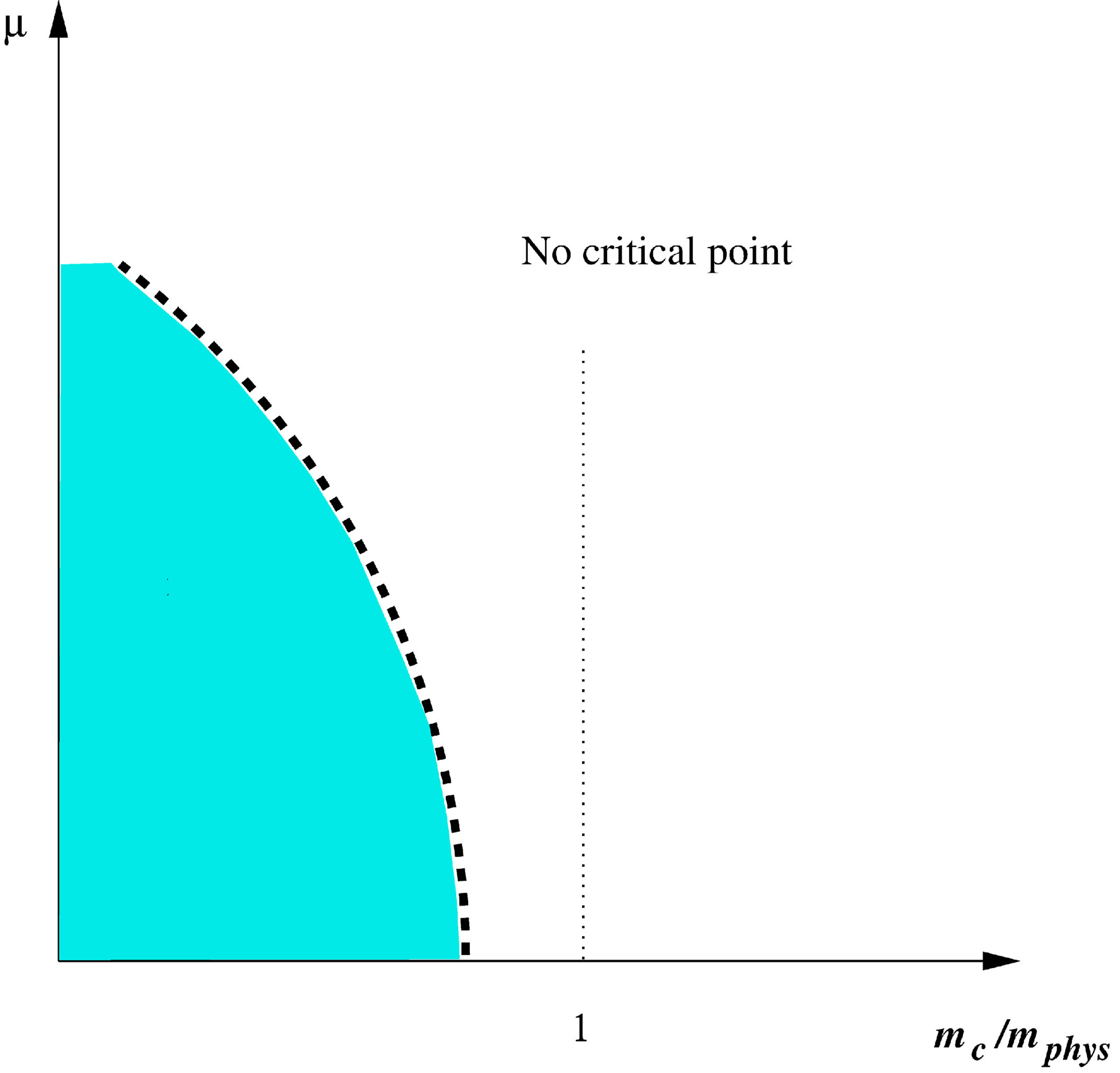
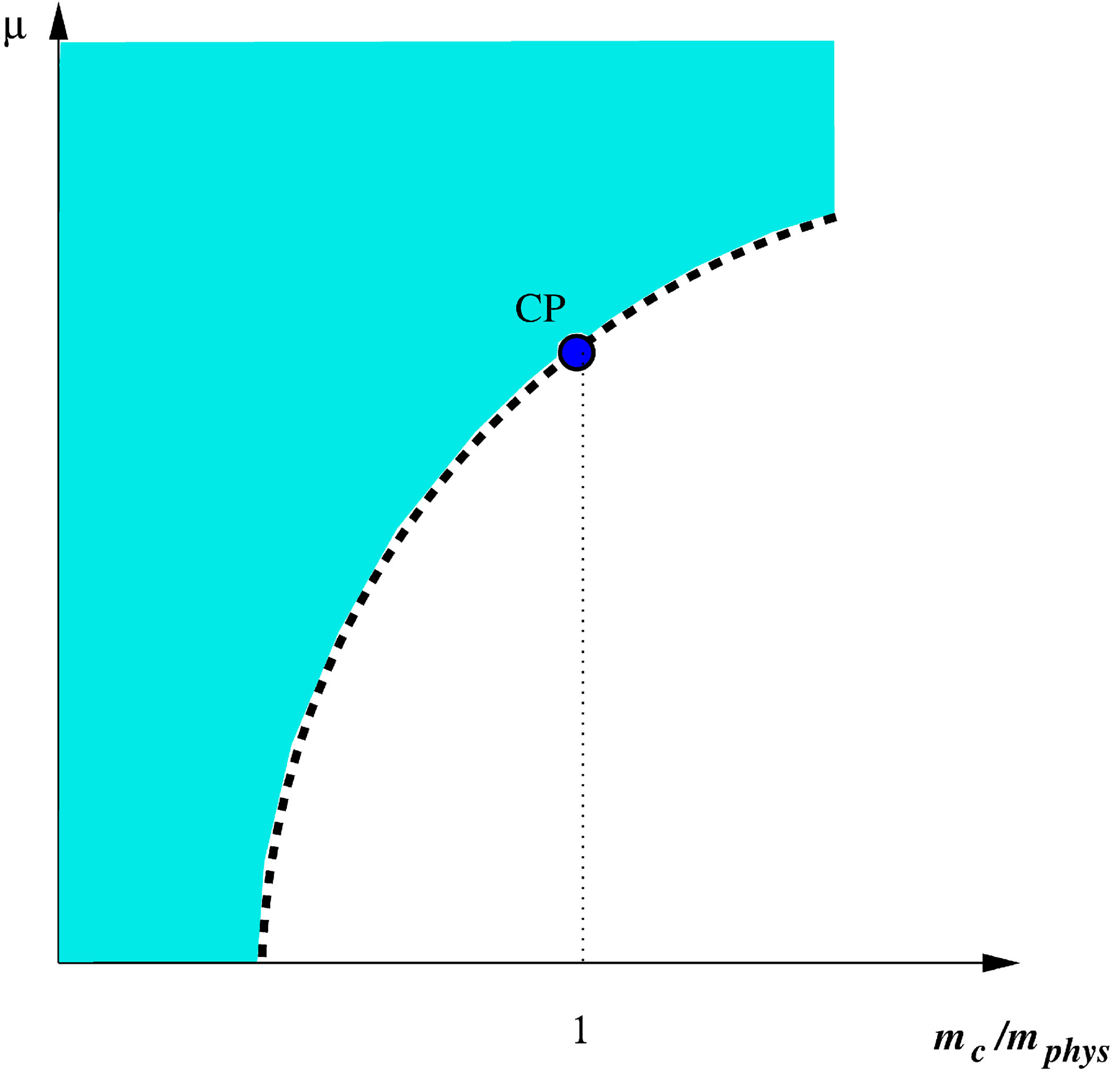
Figure 1. Upper panel: The “exotic” scenario with the shrinkage of the first order transition region which excludes the presence of a CP at the physical point. Bottom panel: The “standard” scenario with the expansion of the first order transition region which provides the appearance of a CP at the physical point.
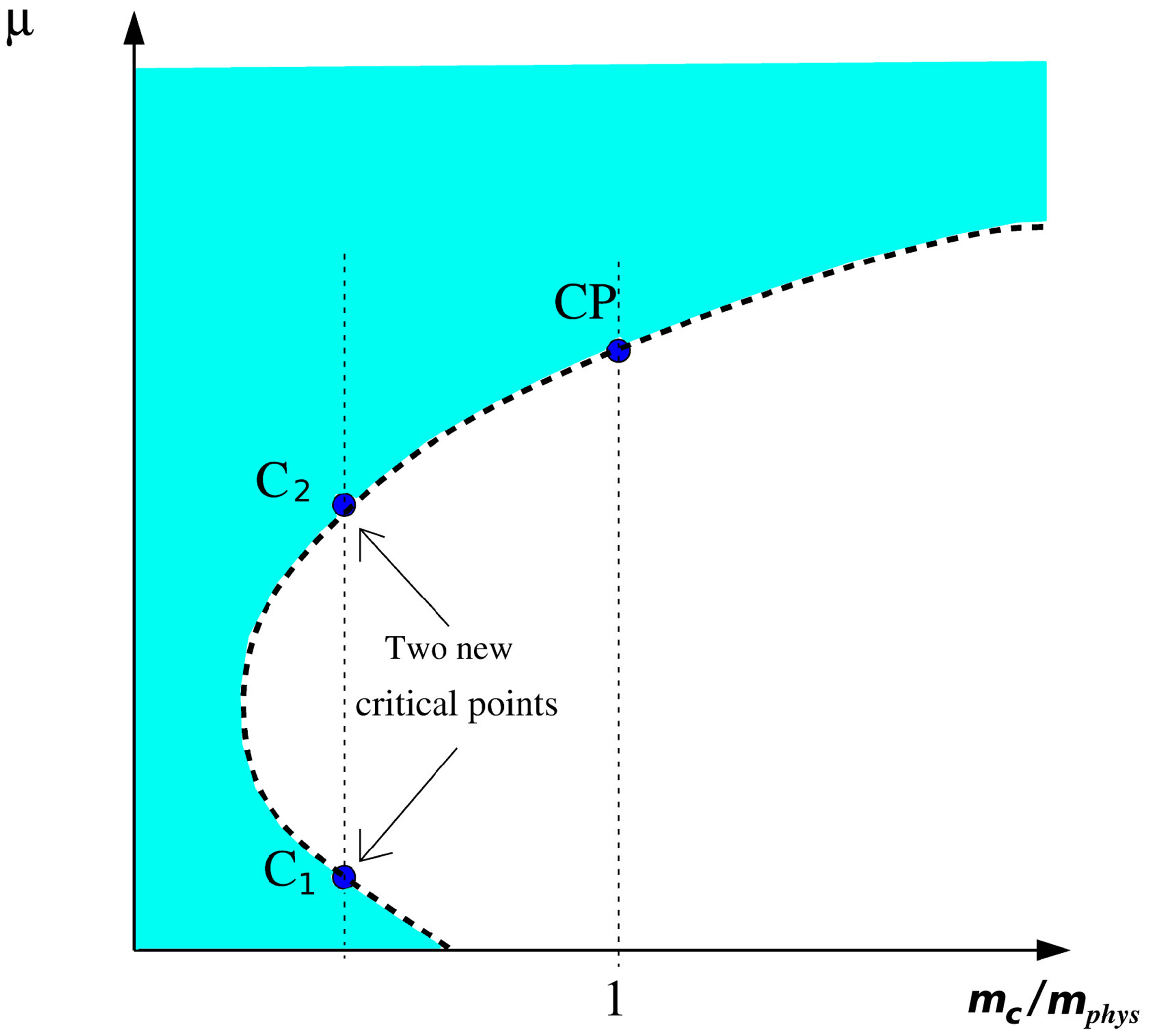
Figure 2. Schematic view of the back-bending scenario in the µ - mc plane. The shaded area represents the region of first order phase transitions; the dashed line represents second order phase transitions while the light part of the figure represents the cross over region. Two critical points (c1 and c2) appear at mc << mphys and the expected CP is present at mc = mphys.
tion lines where one of them represents the usual line which starts at zero temperature and chemical potential of the order of the constituent quark mass while the other is an unusual line which starts at zero chemical potential and high temperature [6,7].
In [4] the author has considered the three flavor Nambu-Jona-Lasinio model (NJL) at large-Nc with an explicit repulsive vector interaction, with coupling GV, in order to produce a back-bending that would conciliate the lattice results obtained by de Forcrand and Philipsen with most model predictions. It is well known that within the NJL this type of interaction weakens the first order transition line [8] in opposition to the scalar coupling  which tends to favor the appearance of first order phase transitions [9] . The explicit presence of a vector term was decisive in order to produce the back-bending scenario within the large-Nc application of [4] . It was explained that the net effect produced by a repulsive vector channel is to add a term like −GV rq2 (here ρq represents the quark number density) to the pressure and as a result the size of the first order covers a smaller range of temperatures as compared to the GV = 0 case.
At the same time, the value of the coexistence chemical potential for a given temperature occurs at a higher value when GV ≠ 0 and, as a consequence, the critical end point happens at smaller temperatures to be higher chemical potentials than in the case of vanishing GV. Although such a vector term is known to be important at high densities in theories such as the Walecka model for nuclear matter, its consideration is more delicate within a non renormalizable model such as the NJL where usually the integrals are regulated by a momentum cut-off, Λ. Within this model, GS and Λ are usually fixed to reproduce the pion mass , the pion decay constant
 and the quark condensate
 which yields Λ ~ 560 - 670 MeV, GS Λ2 ~ 2 - 3.2 and mc ~ 5 - 5.6 MeV (see [10] for a complete discussion).
However, fixing GV poses and additional problem since this quantity should be fixed using the ρ meson mass which, in general, happens to be higher than the maximum energy scale set by Λ. Then, GV is usually considered to be a free parameter whose estimated value ranges between 0.25 GS and 0.5GS [11,12].
Alternatively, when going beyond the large-Nc (or mean field) level one may induce quantum (loop) corrections which mimic the physical effects caused by a classical (tree) term such as GV. This is precisely what has been observed in an application of the nonperturbative Optimized Perturbation Theory (OPT) method to the two flavor NJL model with vanishing GV [13] . The OPT results for phase diagram for this model show that  corrections induced by this approximation reproduce the same qualitative features obtained by considering the model at large-Nc with an explicit repulsive vector channel. The reason is that the OPT two loop contributions add a term like
  to the pressure.
The relationship between the OPT, at GV = 0, and the large-Nc approximation, at GV ≠ 0, has been recently investigated in great detail in the framework of the abelian NJL at finite densities and zero temperature in [14] . In the context of the eventual back-bending behavior of the critical line in the μ − mc plane, the OPT has also been previously employed with success in [7] . There, the strategy was to use very high values for GS in order to obtain a T − μ phase diagram dominated by first order chiral transitions only.
Then, the OPT with its  term was used at different quark mass values showing that, in this case, two critical points emerge at low mc due to the weakening of the first order line at intermediate μ values leading to the back-bending behavior observed in [4] without the need to explicitly include a vector channel in the lagrangian density.
Note that a repulsive vector type of coupling was not explicitly considered in the two flavor LSM application performed by Bowman and Kapusta which, on the other hand, was carried out beyond the mean field level through the consideration of thermal fluctuations.
In the present work, we extend the comparison between the OPT (at GV = 0) and the large-Nc approximation (at GV ≠ 0) to the non abelian NJL model at finite temperature and density in the strong coupling and small quark mass regime showing that, as expected, both methods agree from the qualitative point of view leading to a back-bending which would be completely missed by a standard large-Nc evaluation.
Our results also emphasize the importance played by  terms which are easily taken into account by the OPT so that this method may be viewed as a robust alternative to investigate nonperturbative effects related to the chiral transition of strongly interacting matter. The work is organized as follows. In the next section, we perform a large-Nc application to the two flavor NJL version in the strong coupling regime for the GV ≠ 0 case. In Section 3 we review the OPT results, at GV = 0, which were originally obtained in [7]. We then compare, in Section 4, the analytical and numerical results obtained with the two different model approximations. Our conclusions are presented in Section 5.
2. The NJL in the Strong Coupling Regime
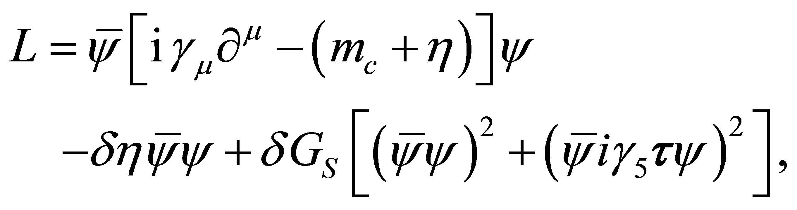
The standard version of the two flavor Nambu-JonaLasinio model lagrangian density L with a repulsive vector channel reads [10,15]
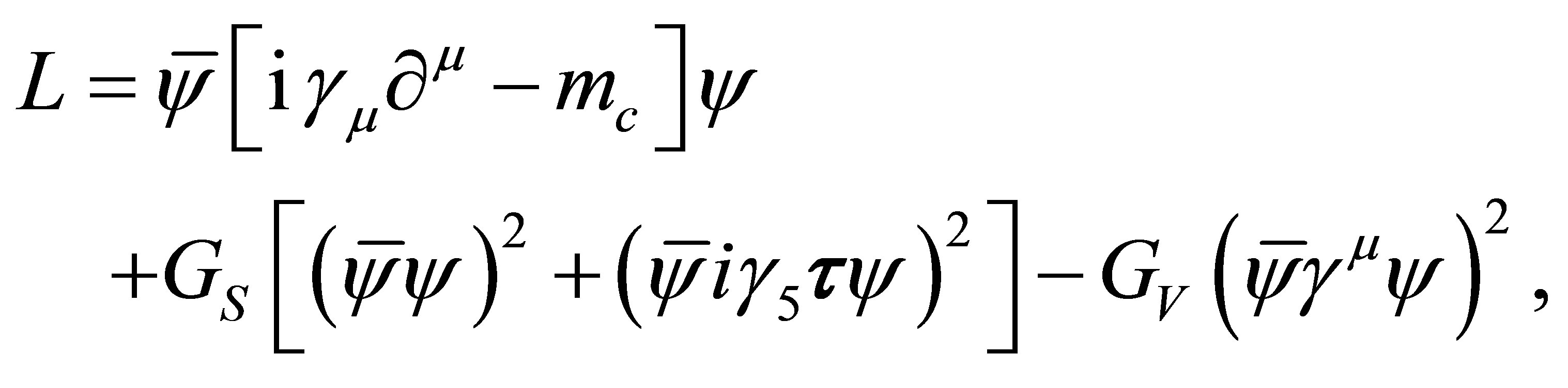 (1)
(1)
where y (a sum over flavors and color degrees of freedom is implicit) represents a flavor isodoublet (u and d type of quarks) Nc-plet quark fields while  are isospin Pauli matrices.
As emphasized in [16] , the introduction of a repulsive vector interaction term of the form  in Equation (1) is also allowed by the chiral symmetry. Such a term can become important at finite densities, generating a saturation mechanism depending on the vector coupling strength that provides better matter stability [10,16]. Here, we will show that this term also influences the phase diagram, especially at the low temperature and high density region. A standard parametrization for this model is Λ = 587.9 MeV, GS Λ2 = 2.44, and mc = 5.6 MeV so that, with these inputs, one obtains fπ = 93 MeV, mπ = 135 MeV, and M = 400 MeV at T = 0, and μ = 0 [10] .
However, as will be shown in the next subsection, in order to simulate the back-bending behavior in the present model we will keep Λ = 587.9 MeV considering  while varying the current quark mass from mc = 0 to mc = mphys= 5.6 MeV. As discussed in [7] this nonstandard choice does not affect very much the predicted values for observables such as fπ , mπ and
 . On the other hand the quark effective mass, which is directly proportional to GS, assumes very high values (around 800 MeV > Λ). However, this is not a problem for our present purpose of simulating the back-bending in a qualitative way (see [7] for a more complete discussion).
2.1. Thermodynamical Potential at Large-Nc with Finite GV Contributions
The large-Nc (or MFA) evaluation of the thermodynamical potential within this model is standard and yields [10]
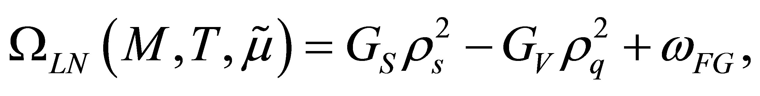 (2)
(2)
where the dressed “free gas” term is given by
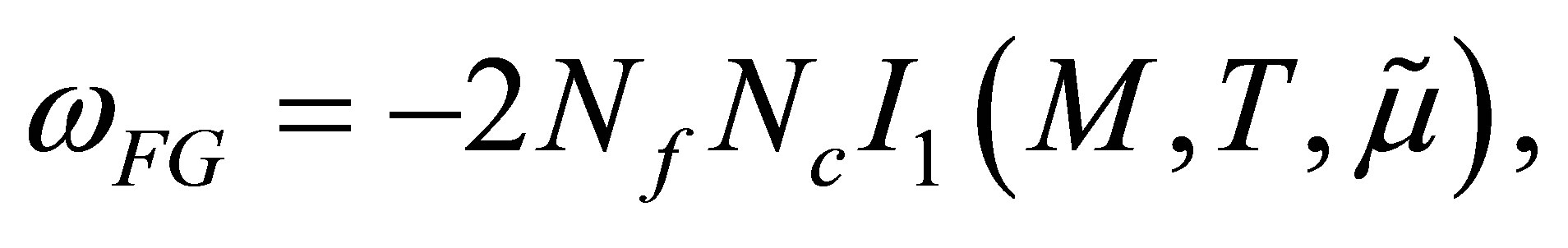 (3)
(3)
the scalar density is given by
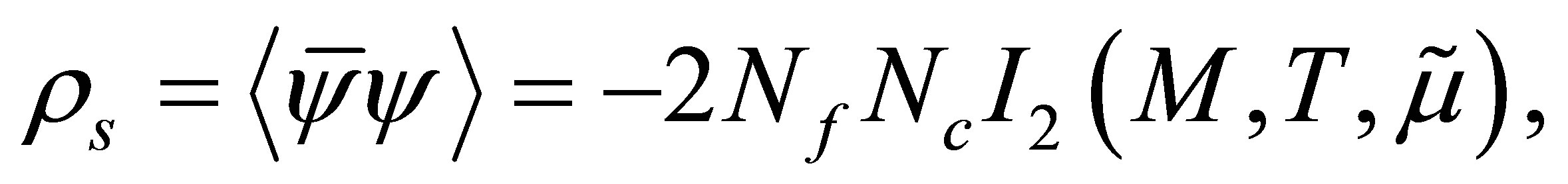 (4)
(4)
and the quark number density is given by
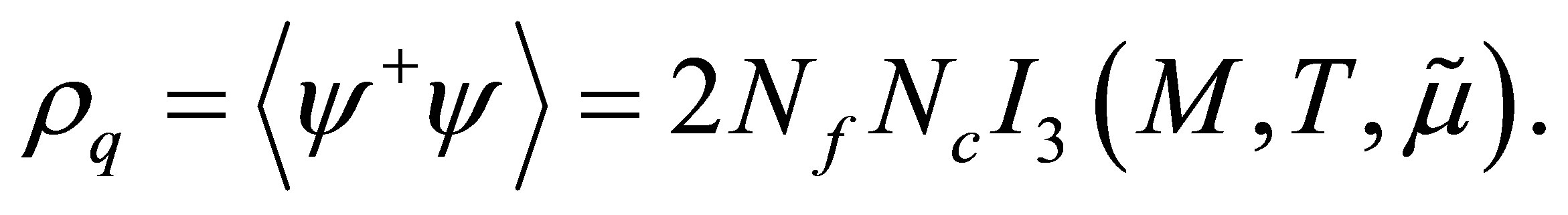 (5)
(5)
The integrals appearing in the above equations are defined by
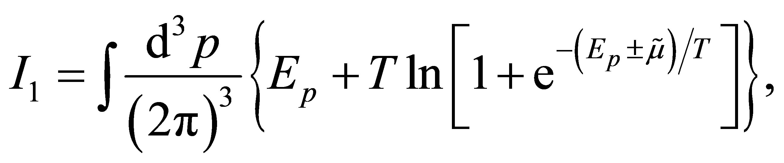 (6)
(6)
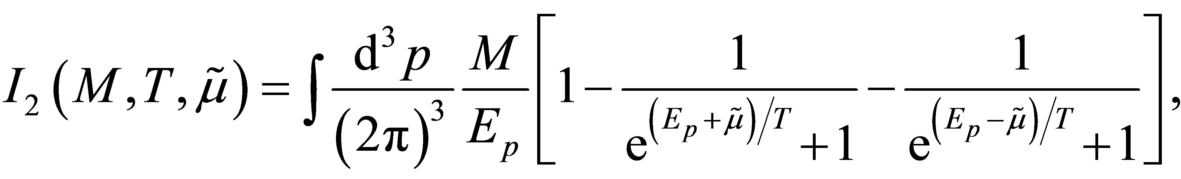 (7)
(7)
and
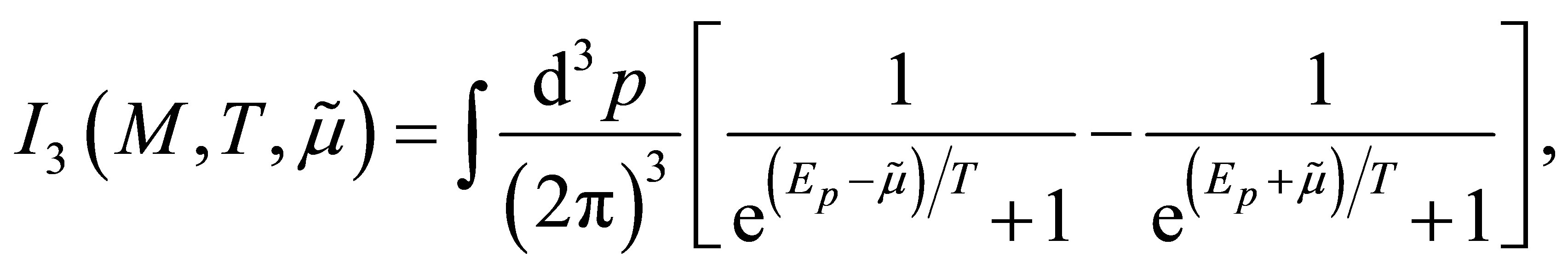 (8)
(8)
where  Here, the divergent contributions corresponding to the first term on the right hand side of Equations (6) and (7) are regulated by Λ. The effective quark mass, M, and the effective chemical potential, µ, are obtained from solving the following coupled self consistent equations
 (9)
(9)
and
 (10)
(10)
Let us now review the main effects of the repulsive vector interaction in the phase diagram by considering the standard parametrization. Figure 3 shows the situation for GS Λ2 = 2.44, Λ = 587.9 MeV and mc = 0 (chiral limit) at GV /GS = 0, 0.1, and 0.4. As expected the GV term has little effect at low chemical potential values where the second order chiral transition dominates since mc = 0.
One also notices that, as GV increases, the first order chiral transition line weakens so that the tricritical point occurs at smaller temperatures. It is also clear that for a given temperature the coexistence chemical potential takes place at higher values with increasing GV. This scenario is also observed away from the chiral limit  except that now the second order transition is replaced by a cross over region and the tricritical point turns into a critical end point. This type of phase diagram where a CP naturally appears at the physical quark mass point is predicted by most model approximations. Now, in order to simulate the lattice results by de Forcrand and Philipsen we first need to obtain a first order phase transition at μ = 0 for low mc values so that at vanishing densities our results would be consistent with the lattice results furnished by the Columbia plot [17] .
Within the NJL this is easily achieved by increasing GS [9] so that, at GV = 0 and mc = 0, the whole phase diagram is dominated by a first order phase transition. Figure 4 shows this situation in the strong coupling regime for different values of GV and mc. Let us first analyze the case GV = 0 by noticing that if one increases mc the first order line weakens and turns into a cross over at μ = 0. Figure 5 illustrates the situation in the μ − mc
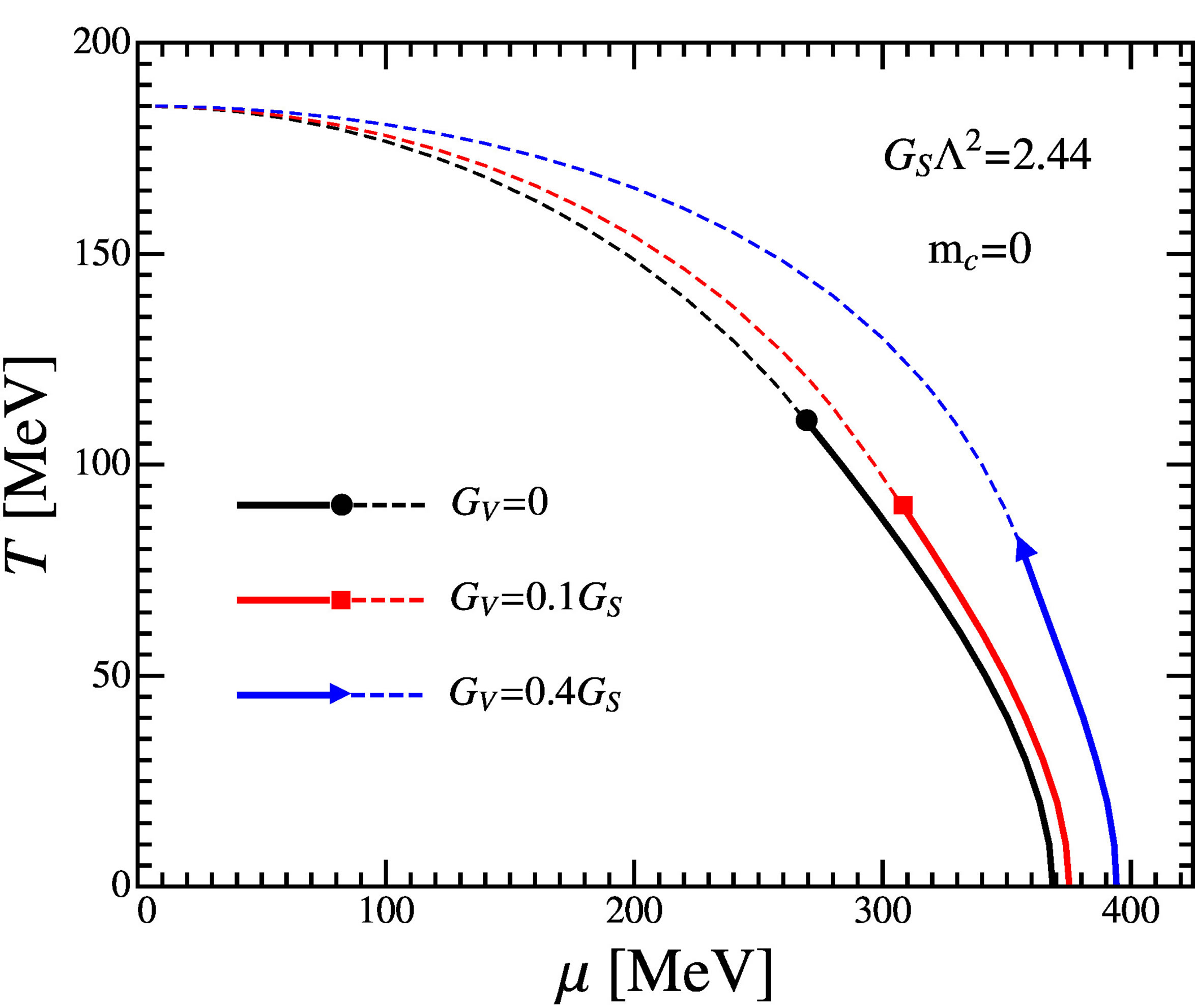
Figure 3. The large-Nc phase diagram for a standard parametrization (L = 587.9 MeV and GSL2 = 2.44) in the chiral limit (mc = 0). The continuous lines represent first order phase transition and the dashed lines represent second order phase transitions. The solid symbols represent the tricritical points for the ratios GV/GS = 0, 0.1 and 0.4. Note that GV weakens the first order phase transition and, for a given T, shifts the coexistence chemical potential to higher values.

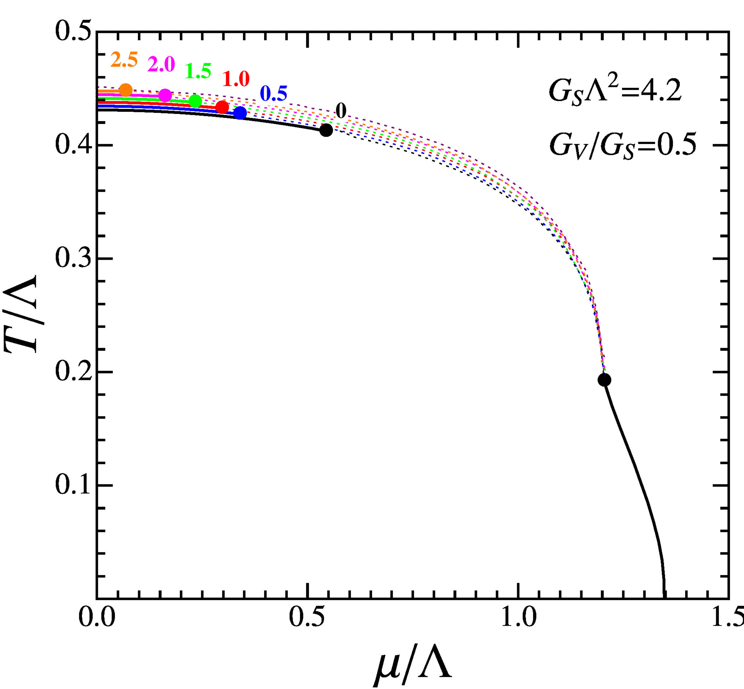
Figure 4. The large-Nc phase diagram in the strong coupling regime (L = 587.9 MeV and GSL2 ³ 4). Upper panel: the chiral limit (mc = 0) where the continuous lines represent first order phase transitions and the dashed lines represent second order phase transitions. The solid symbols represent the tricritical points for the ratios GV/GS = 0, 0.1 and 0.3. Bottom panel: different current mass values (mc/mphys = 0, 0.5, 1.0, 1.5, 2.0 and 2.5) have been used with fixed GV/GS = 0.5. For mc ≠ 0 the dashed lines represent the cross over region. Both panels show that GV weakens the first order phase transition but for small mc and high GS its presence leads to the emergence of two (tri) critical points. Note how mc has a greater influence over the high-T region while GV affects the intermediate to low-T region.
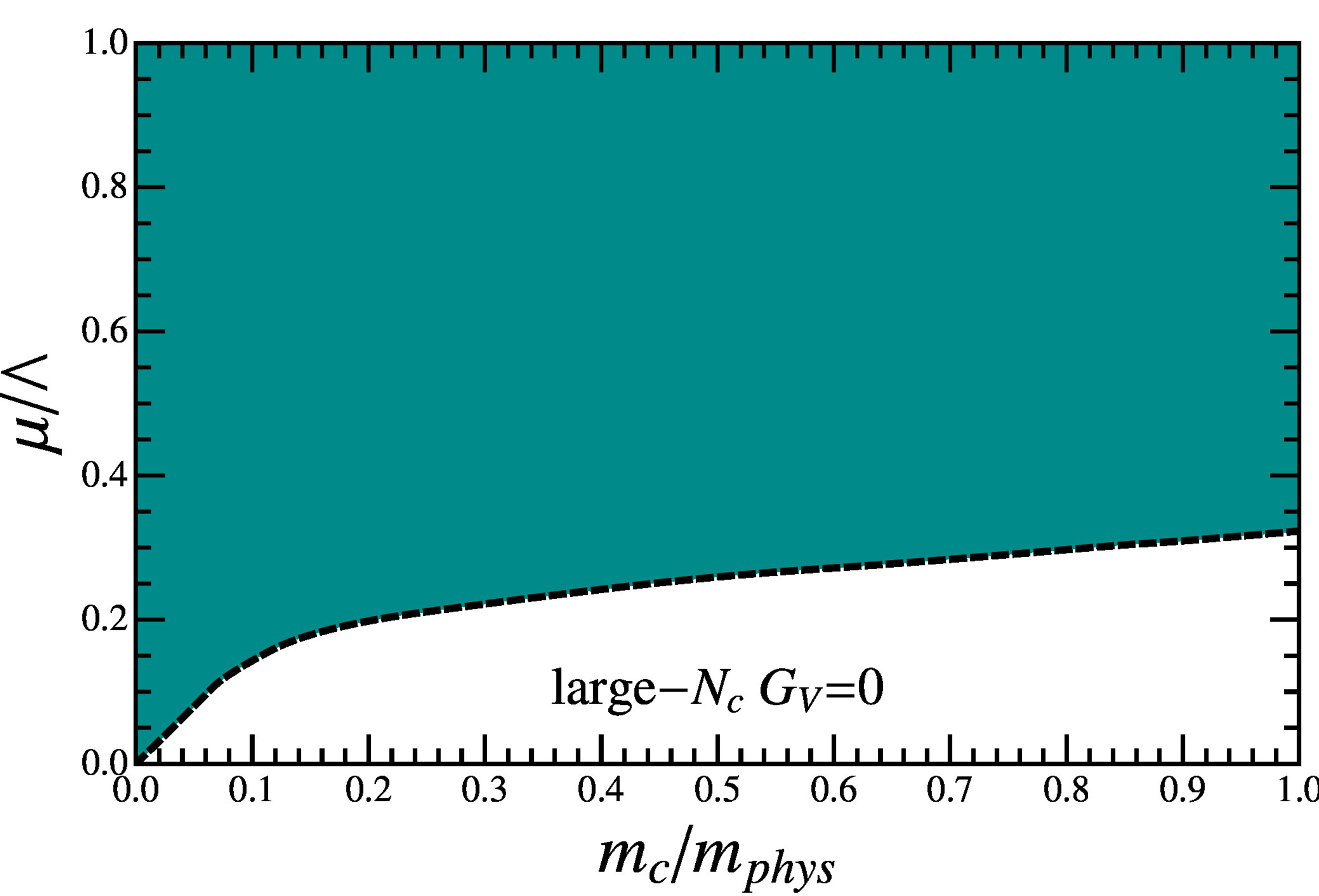
Figure 5. The µ − mc plane, at large-Nc for GV = 0 at strong (scalar) coupling (L = 587.9 MeV, GSL2 = 4). The shaded area represents the region of first order phase transitions; the dashed dark line represents second order phase transitions while the light part of the figure represents the cross over region. The figure shows that there is no back-bending scenario at large-Nc when GV = 0.
plane showing that, for GV = 0, the first order line recedes from the temperature axis as mc increases without reproducing the back-bending scenario which would conciliate the de Forcrand and Philipsen results with model predictions. Now, if we turn on the vector interaction, still at mc = 0, the weakening of the first order transition happens in a different way so that two segments of first order chiral transitions appear. One of them is the usual one which starts at T = 0 while the other is an unusual first order line which starts at μ = 0 as Figure 4 shows. So, at the expense of considering a strong GS and a finite GV we have managed to induce the appearance of two tricritical points at vanishing mc which, as will be shown in Section 3, leads to the back-bending scenario.
2.2. Thermodynamical Potential at Vanishing GV with Finite Nc Contributions
The basic idea of the OPT method is to deform the original lagrangian density by adding a quadratic term like  to the original lagrangian density as well as by multiplying all coupling constants by δ [7] . The new parameter δ is just a bookkeeping label and η represents an arbitrary mass parameter. Perturbative calculations are then performed in powers of the dummy parameter δ which is formally treated as small and set to the original value, δ = 1, at the end1.
Therefore, the fermionic propagator is dressed by η which may also be viewed as an infrared regulator in the case of massless theories. After a physical quantity, such as the thermodynamical potential (Ω), is evaluated to the k-order and δ set to the unity only a residual η dependence remains. Then, optimal nonperturbative results can be obtained by requiring that Ω(k) (η) be evaluated where it is less sensitive to variations of the arbitrary mass parameter. This requirement translates into the criterion known as the Principle of Minimal Sensitivity (PMS) [18]
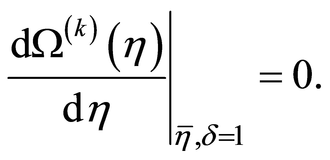 (11)
(11)
In general, the solution to this equation implies in self consistent relations generating a nonperturbative coupling dependence. In most cases nonperturbative  corrections appear already at the first nontrivial order while the large-Nc (or MFA) results can be recovered at any time simply by considering Nc → ∞. Finally, note that the OPT has the same spirit as the Hartree and the Hartree-Fock approximation in which one also adds and subtracts a mass term. However, within these two traditional approximations the topology of the dressing is fixed from the start: direct (tadpole) terms for Hartree and direct plus exchange terms for Hartree-Fock. On the other hand, within the OPT, the dressed mass term
  acquires characteristics which change order by order progressively incorporating direct, exchange, vertex corrections, etc, effects. The differences between these three different methods have been recently discussed in [14] . To implement the OPT within the NJL model at GV = 0 one follows the prescription used in [13] to write
 (12)
(12)
Then, the order-δ thermodynamical potential can be written as (see [13] for technical details)
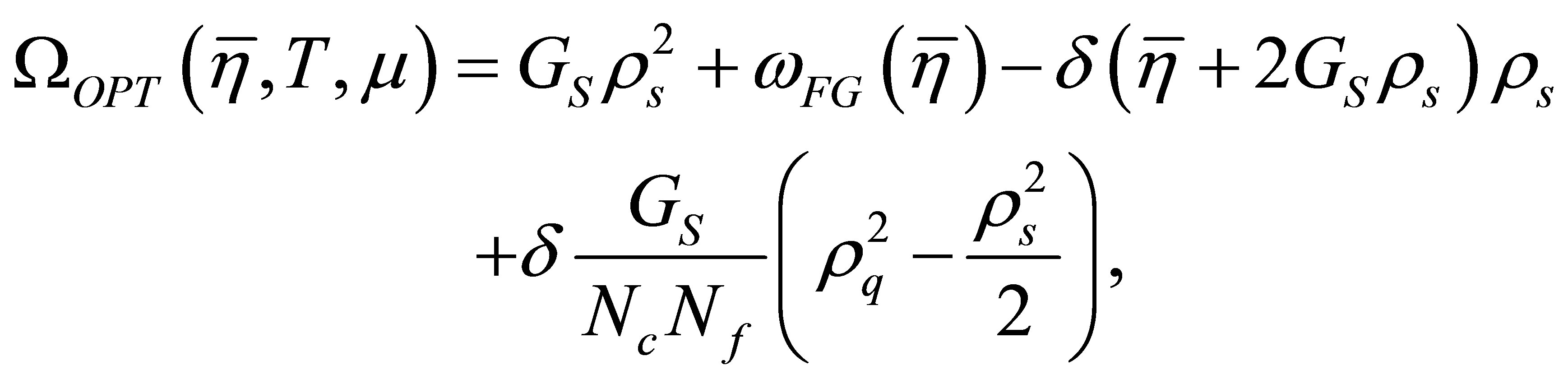 (13)
(13)
where now all the integrals  defining the quantities ωFG, ρs , and ρq are redefined as
 . Then, for each pair of
  values the optimum mass parameter,
  , can be obtained by solving the PMS equation given by [13]
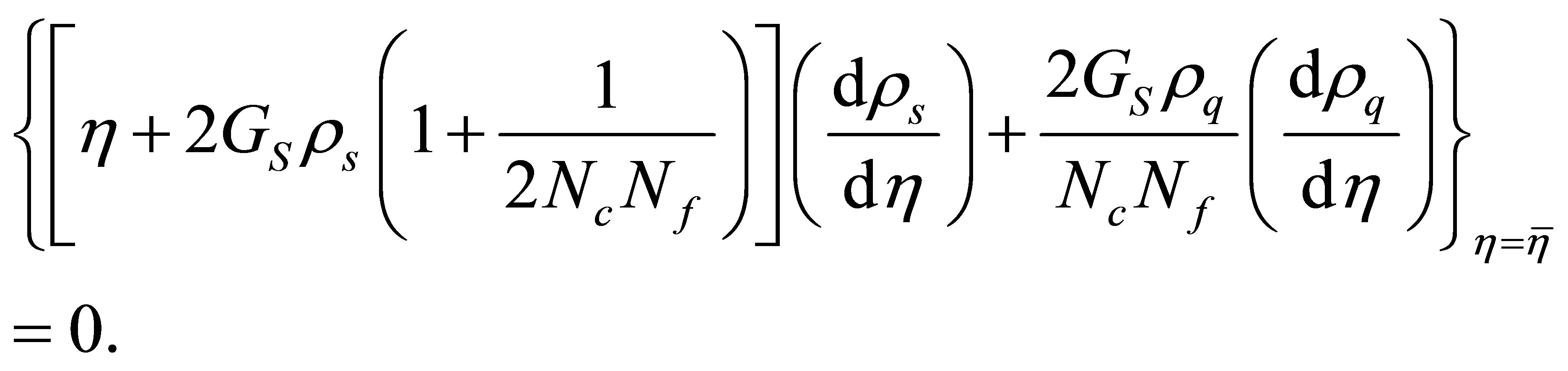 (14)
(14)
Note that when Nc → ∞ the PMS optimization procedure sets  = −2GSρs exactly reproducing the large-Nc result (for the standard NJL model) with no ρq dependence. By comparing the OPT thermodynamical potential given by Equation (13) with its large-Nc counterpart given by Equation (2) one notices that the OPT induces a finite Nc correction of the form
  while, as discussed in [4] , the GV term gives a net contribution of the form GV ρq2. Then, one could expect that the two different model approximations given by the OPT (at GV = 0) and the large-Nc approximation (at GV ≠ 0) lead to the same qualitative picture of the phase diagram. A recent comparison performed with one flavor at vanishing temperature in [14] showed that this is indeed the case.
Here, we are now in position to extend that comparison to the more realistic two flavor case at finite temperatures.
3. Comparing the OPT at GV = 0 with the Large-Nc Approximation at GV = 0
Let us now compare the results furnished by the two approximations for the NJL model at high GS. Figure 6 shows the T − μ phase diagram when chiral symmetry is weakly broken . This figure also shows the large-Nc result for GV = 0 which predicts a first order transition taking place in the whole plane. At the same time the OPT with its
  contribution and the large-Nc at GV ≠ 0 weaken that line at intermediate chemical potential values so that two critical points appear in this case of small current mass as expected from the discussion related to Figure 2. Then, by varying the mc values towards the physical one (mphys) one can map the T − μ diagram into the μ − mc plane as shown in Figure 7. This figure clearly shows that both approximations considered here manage to produce the back-bend-
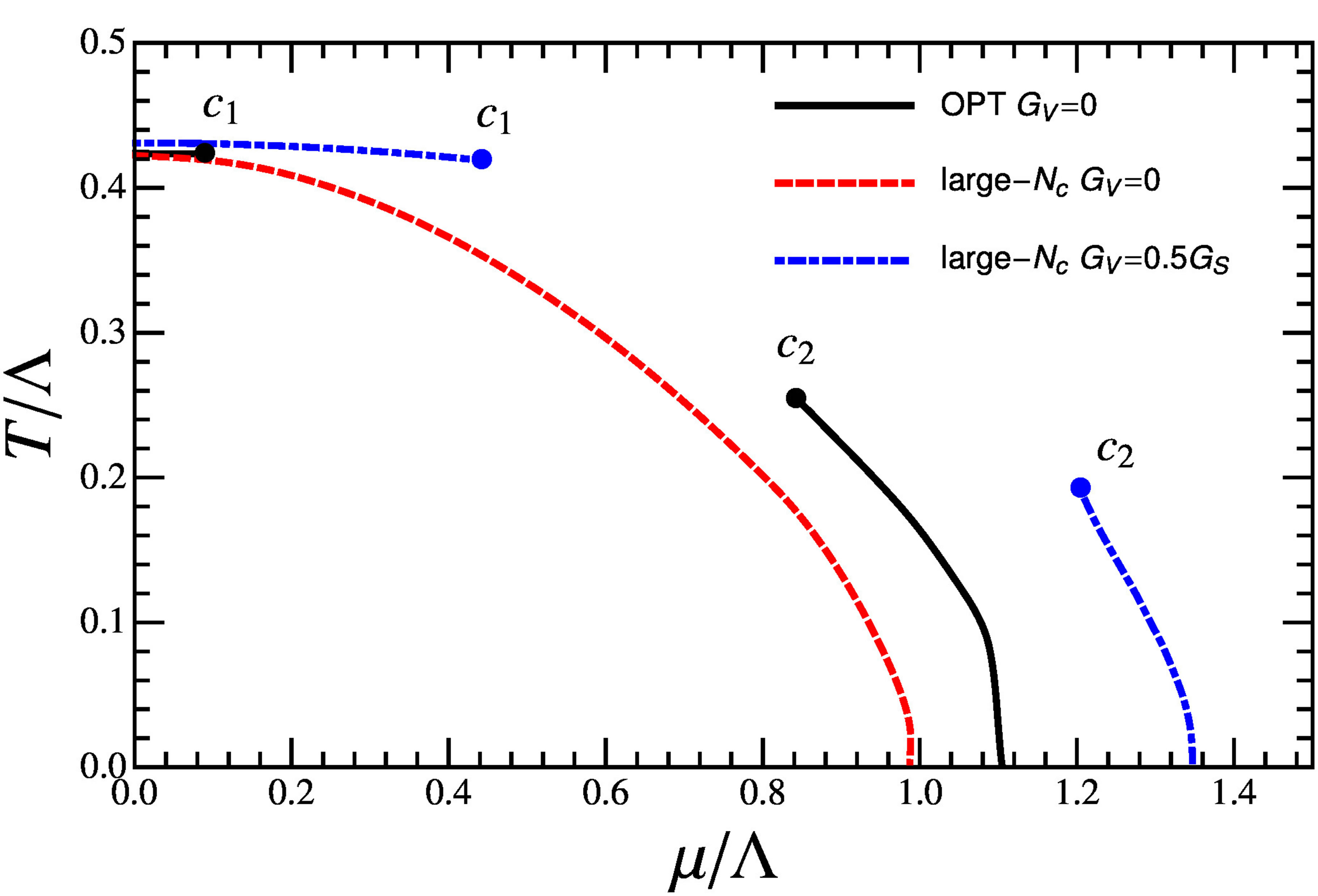
Figure 6. The large-Nc (at GV/GS = 0.5) and the OPT (at GV = 0) phase diagrams in the strong coupling regime (L = 587.9 MeV and GSL2 = 4) for weakly broken chiral symmetry (mc = 0.1 MeV). The figure shows the usual CP (c2) and the exotic high-T CP (c1) at the end of the first order transitions for the OPT (continuous line) and large-Nc (dotdashed). For comparison the figure also shows the large-Nc result (at GV = 0 and mc = 0) with the dashed line representing the first order transition.
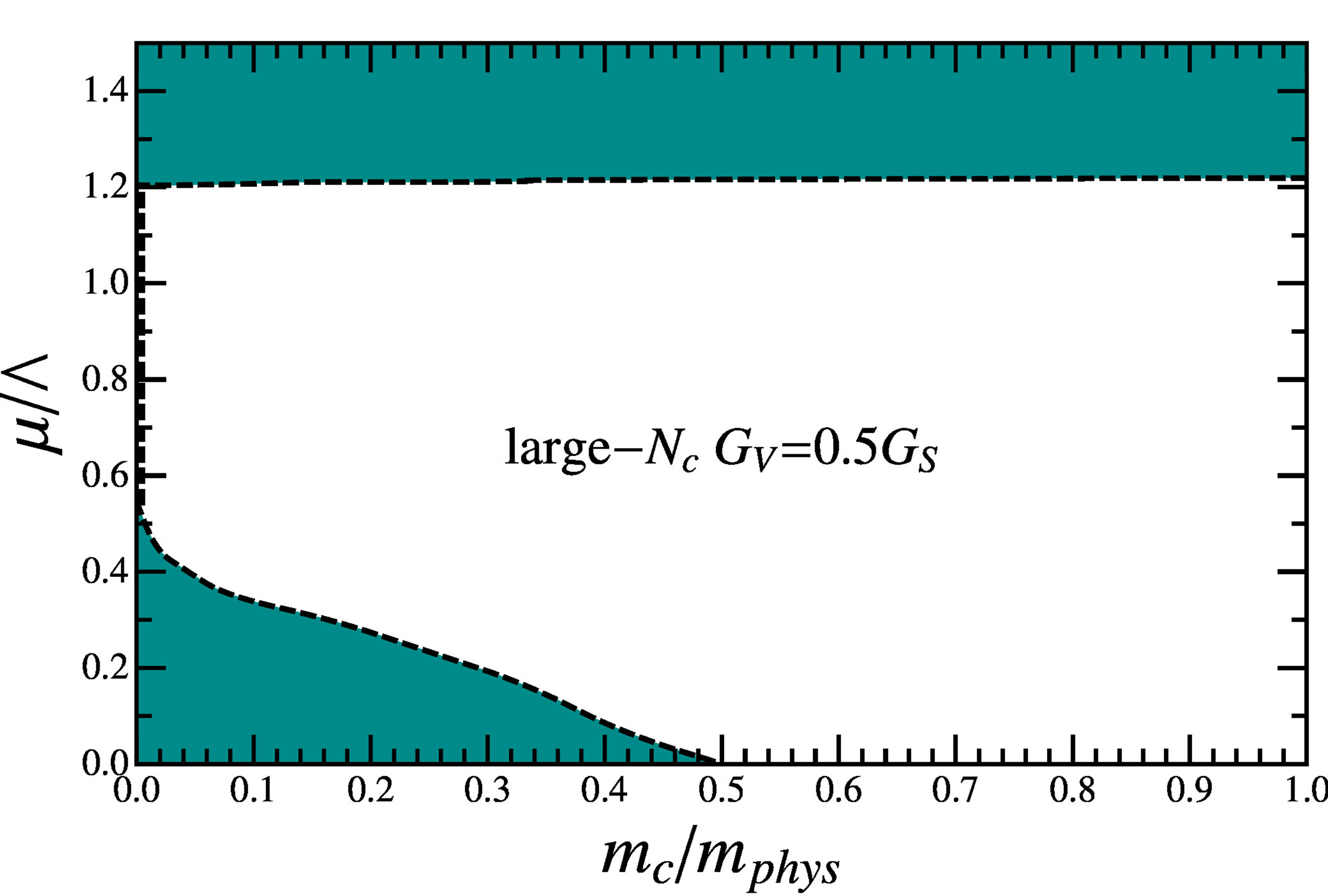
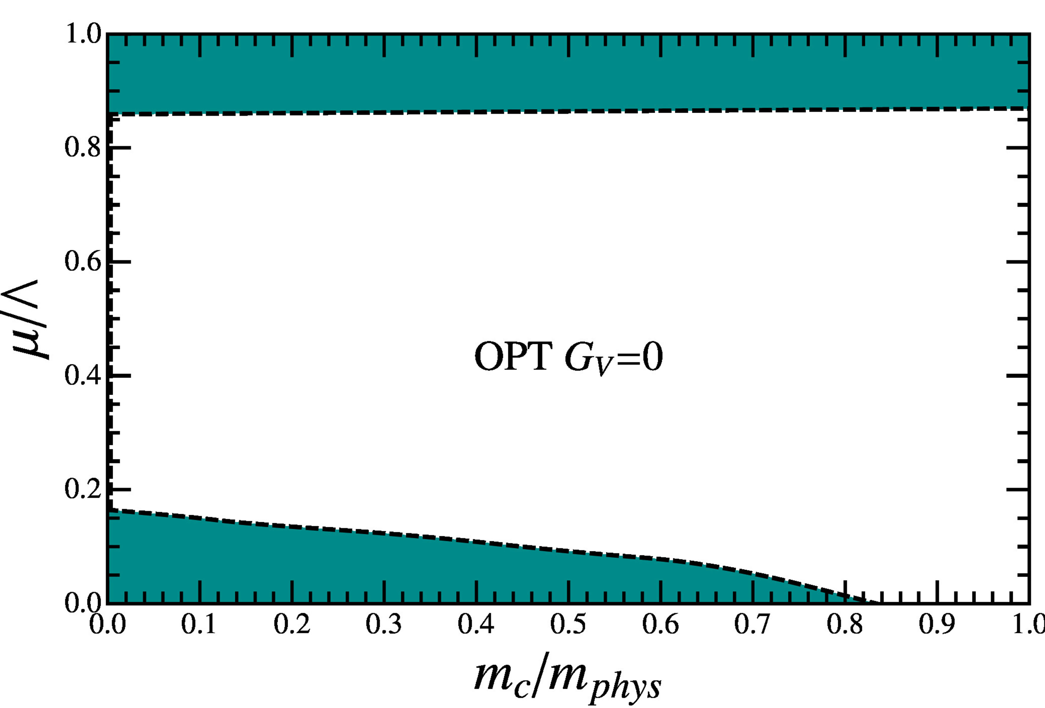
Figure 7. The µ − mc plane at strong (scalar) coupling (L = 587.9 MeV, GSL2 = 4) showing the back-bending. The shaded area represents the region of first order phase transitions; the dashed dark line represents second order phase transitions while the light part of the figure represents the cross over region. Left panel: The large-Nc result at GV/GS = 0.5. Right panel: The OPT result at GV = 0. In both cases one observes two CP at mc << mphys but only the one at high µ survives at the physical point (mc = mphys).
ing of the critical line so that the CP will be recovered at mc = mphys even if initially (at low values of μ) the line bends in such a way which is reminiscent of the “exotic” scenario displayed by the right panel of Figure 1. The physical nature and even the critical exponents of the two different critical points which occur at small mc have been discussed in great detail in [7] . From our results it is clear that as mc → mphys the unusual first order line disappears and only the usual “liquid-gas” type of first order line survives in accordance with most model predictions.
4. Conclusions
We have considered the two flavor NJL model in the strong scalar coupling regime (GSΛ2 @ 4) in order to compare two distinct model approximations. The first is the traditional large-Nc approximation which was applied by explicitly considering a finite repulsive vector interaction (proportional to GV) which was introduced at the classical (tree) level. The second is the alternative OPT method which was applied to the standard version of the NJL model .
.
Our first step towards the simulation of the backbending behavior was to tune GS at GV = 0 so that the large-Nc approximation predicts that the first order transition line, which usually starts at T = 0, will touch the T axis at μ = 0 for very small mc values.
For mass values closer to the physical ones, this approximation recovers the expected cross over behavior at small μ with the appearance of a single critical point at intermediate chemical potentials. Next, we have shown that by considering finite values for GV at  this single first order transition line splits into two lines in the T − μ plane. One of them is similar to the usual “liquid-gas” line which starts at T = 0 and ends at intermediate temperature values. The other one, which has a more “chiral” behavior according to the analysis of [7] , is located at the high temperature region and disappears as mc approaches mphys from below. In this way, we were able to induce the back-bending behavior for two flavors in a manner analogous to the one adopted in [4] for the three flavor case. The OPT results for this strong coupling and small regime obtained in [7] were then reviewed so that a numerical comparison could be performed. At the first non trivial order, this approximation includes one and two loop terms which would belong to the
  and
and  in the usual
  type of expansion. In particular, the two loop terms generate a negative contribution to the pressure given by
  , where ρq represents the fermionic density. This term is similar to the net −GV ρq2 contribution considered at large-Nc [4] . Within the OPT the
  suppressed vector term competes with its scalar counterpart, ρs, weakening the first order line at intermediate values of μ and enhancing the appearance of two critical points in the T − μ plane for mc values which are smaller than the physical ones. Finally by scanning the values of mc, we have mapped the T − μ phase diagram into the μ − mc plane observing that, for strong couplings, the large-Nc approximation, at finite GV , and the OPT, at vanishing GV , predict that the first order transition region shrinks for low values of μ as observed in the lattice simulations of [1]. But then, at intermediate chemical potentials, the vector terms −GV ρq2 (large-Nc) and
  (OPT) change the first order phase transition region into a cross over region. Finally, at higher chemical potentials, the first order transition region reappears and then expands as μ is increased. So, our results suggest that even if an initial shrinkage of the first order region is confirmed by lattice simulations, it does not necessary rule out the existence of the CP which is expected to occur at intermediate chemical potentials for physical quark masses. In this case, a back-bending will be observed on the μ − mc plane outlining the importance of a repulsive vector contribution in agreement with [4] . Our comparison allows us to conclude that similar qualitative results will be obtained either by explicitly considering such a contribution at the classical level as in the large-Nc case or by radiatively generating it by going beyond the mean field level. Within the NJL model, the advantage of the second procedure, which can easily be implemented within the OPT, is that it does not require the fixing of GV which is a drawback of the first procedure. The results obtained in the present application support those obtained in [14] , for the simpler abelian NJL model at vanishing temperature, showing the robustness of the OPT method. Finally, note that at these non standard high coupling values our results are to be taken only as qualitative predictions.
5. Acknowledgements
This work was partially supported by CAPES, CNPq and FAPESC (Fundação de Amparo à Pesquisa e Inovação do Estado de Santa Catarina).
REFERENCES
- P. de Forcrand and O. Philipsen, Journal of High Energy Physics, Vol. 0811, 2008.
- P. de Forcrand and O. Philipsen, Journal of High Energy Physics, Vol. 0701, 2007.
- P. de Forcrand, S. Kim and O. Philipsen, “A QCD Chiral Critical Point at Small Chemical Potential: Is It There or Not?” Proceedings of the 25th International Symposium on Lattice Field Theory, Regensburg, 30 July-4 August 2009.
- K. Fukushima, Physical Review D, Vol. 78, 2008, Article ID: 114019. http://dx.doi.org/10.1103/PhysRevD.78.114019
- V. Koch, “Exploring the QCD Phase Diagram: Fluctuations and Correlations,” Proceedings of the 5th International Workshop on Critical Point and Onset of Decon- finement, Long Island, 8-12 June 2009.
- E. S. Bowman and J. I. Kapusta, Physical Review C, Vol. 79, 2009, Article ID: 015202. http://dx.doi.org/10.1103/PhysRevC.79.015202
- L. Ferroni, V. Koch and M.B. Pinto, Physical Review C, Vol. 82, 2010, Article ID: 055205. http://dx.doi.org/10.1103/PhysRevC.82.055205
- K. Fukushima, Physical Review D, Vol. 77, 2008, Article ID: 114028. http://dx.doi.org/10.1103/PhysRevD.77.114028
- S. P. Klevansky, Reviews of Modern Physics, Vol. 64, 1992, pp. 649-708. http://dx.doi.org/10.1103/RevModPhys.64.649
- M. Buballa, Physics Reports, Vol. 407, 2005, pp. 205-376. http://dx.doi.org/10.1016/j.physrep.2004.11.004
- S. Carignano, D. Nickel and M. Buballa, Physical Review D, Vol. 82, 2010, Article ID: 054009. http://dx.doi.org/10.1103/PhysRevD.82.054009
- R. Rapp, T. Schafer, E. V. Shuryak and M. Velkovsky, Physical Review Letters, Vol. 81, 1998, pp. 53-56. http://dx.doi.org/10.1103/PhysRevLett.81.53
- J.-L. Kneur, M. B. Pinto and R. O. Ramos, Physical Review C, Vol. 81, 2010, Article ID: 065205. http://dx.doi.org/10.1103/PhysRevC.81.065205
- J.-L. Kneur, M. B. Pinto, R. O. Ramos and E. Staudt, International Journal of Modern Physics E, Vol. 21, 2012, Article ID: 1250017. http://dx.doi.org/10.1142/S0218301312500176
- Y. Nambu and G. Jona-Lasinio, Physical Review, Vol. 124, 1961, pp. 246-254. http://dx.doi.org/10.1103/PhysRev.124.246
- V. Koch, T. S. Biro, J. Kunz and U. Mosel, Physics Letters B, Vol. 185, 1987, pp. 1-5. http://dx.doi.org/10.1016/0370-2693(87)91517-6
- K. Fukushima and T. Hatsuda, Reports on Progress in Physics, Vol. 74, 2011, Article ID: 014001. http://dx.doi.org/10.1088/0034-4885/74/1/014001
- P. M. Stevenson, Physical Review D, Vol. 23, 1981, pp. 2916-2944. http://dx.doi.org/10.1103/PhysRevD.23.2916
NOTES
1Recall that within the large-Nc one performs an expansion in powers of 1/Nc where Nc is formally treated as large but set to the original value (Nc = 3 in our case) at the end.