Journal of Modern Physics
Vol.3 No.11(2012), Article ID:24434,5 pages DOI:10.4236/jmp.2012.311213
Kinetical Inflation and Quintessence by F-Harmonic Map
1Faculté des Sciences et Techniques, Université d’Abomey-Calavi, Cotonou, Bénin
2University of Namur, Namur, Belgium
Email: kanfon@yahoo.fr, d.lambert@fundp.ac.be
Received August 2, 2012; revised September 5, 2012; accepted September 15, 2012
Keywords: F-Harmonic Maps; Kinetical Inflation; Kinetical Quintessence
ABSTRACT
We were interested, along this work, in the phenomena of the quintessence and the inflation due to the F-harmonic maps, in other words, in the functions of the scalar field such as the exponential and trigo-harmonic maps. We showed that some F-harmonic map such as the trigonometric functions instead of the scalar field in the lagrangian, allow, in the absence of term of potential, reproduce the inflation. However, there are other F-harmonic maps such as exponential maps which can’t produce the inflation; the pressure and the density of this exponential harmonic field being both of the same sign. On the other hand, these exponential harmonic fields redraw well the phenomenon of the quintessence when the variation of these fields remains weak. The problem of coincidence, however remains.
1. Introduction
1.1. The Cosmological Constant and Its Application
The cosmological constant is the energy density associated to the vacuum. Its presence modifies the property of the space time and the matter. When we consider a homogenous universe, we can put the cosmological equation in the form
 (1)
(1)
where ,
,  ,
,  ,
,  denote respectively the rate of the nonradiative energy, radiative energy, the curvature contribution, the cosmological constant contribution,
  is the scale factor and
 , the present Hubble constant. From this equation, one can deduce some remarks:
• The lenght scale associated to the cosmological scale [1] . This value is too small comparatively to fondamental interaction scale.
• By Equation (1),  and
and  vary in the same way; so if
  is large,
  is big too. But at the very earlier epoch of the universe, when
  how does
  behave?
• From different mesures, we can write  .
.
• It follows from the previous remarks that  is perhaps a dynamical quantity.
1.2. Inflation
The first theory in this domain is the standard hot universe. According to this theory, the universe has been expanding and gradually cooling from a state with infinite temperature and density. In this standard scenario, it is usually assumed, in the very early stages of evolution of the universe, that was very flat and the evolution law is given by
 (2)
(2)
Despite the great phenomegical success of the standard hot universe scenario, this scenario was still somewhat incomplete. We give here some problems arising from this scenario.
• The flatness problem: The universe would be closed and it would have collapsed millions of years ago or the universe would be opened and the present energy density of the universe would be negligible;
• The singularity problem: From Equation (2) it follows that the scale factor of the universe  vanishes at
  whereas the energy density becomes infinitely large;
• The homogeneity and isotropy problems: It was assumed that the universe was initially absolutely homogenous and isotropic. Meanwhile, even at present, the universe is not totally homogenous and isotropic, at least at a sufficiently small lenght scale;
• The galaxy formation problem: It was not quite clear what was the source which generates galaxies;
• The inflationnary universe: According to this, in the very earlier stages, the expansion of the universe was exponential from an instable vacuum state. At the end of this state, the energy of this state transforms itself in energy of hot universe. This theory suppose that, there was a time when the pressure was negative and the negative pressure happens due to a single new real scalar field . In this case the energy and the pressure densities can be written
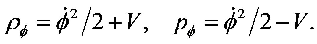 (3)
(3)
If the potential energy V is a slowly varying function of the field  and if the initial value of the time derivation of
  is not too large, the kinetic energy
  can be small compared to
 . If in addition
  is large enough to make a significant contribution to the stressenergy tensor, the pression can satisfy the inflation condition.
1.3. Quintessence
Quintessence has been proposed as the missing energy component that must be added to the baryonic and the matter density in order to reach the critical density [2], [3]. It is a dynamical, slowly-evolving, spatially, inhomogenous component with negative pressure. For quintessence, the equation of state , lies between 0 et –1. A key problem with quintessence proposal is explaining why
  and the matter energy density should be comparable today. One of the aspect to this problem is the coincidence problem [4]. To avoid this problem, Zlatev and al [5] introduce the so-called tracker field. Tracker field have an equation of motion rapidly converge to a common, cosmic evolutionnary track. The tracking solution to which general solutions converge has the property that
  is nearly constant and lies between
  and
and .
.
2. Kinetically Driven Inflation
We consider the following action of a single scalar field minimally coupled with gravity
 (4)
(4)
where ,
,  ,
,  denote the background matter lagrangian and F the contribution of the scalar field. From the action (4), we get the Einstein equation
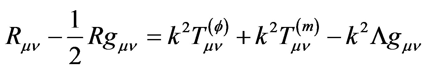 (5)
(5)
and the field equation
 (6)
(6)
The kinetically driven inflation idea is based on the following: Suppose that during the inflationnary epoch, the density of the background matter is negligeable comparatively to the scalar density, and note that the energy and pression densities  and
and  repectively, one can combine the cosmological equations to obtain
 (7)
(7)
To solve Equation (7), Armendariz-Picon and al [6] have looked at the graph of the curve . They observed that the energy density
  grows below the line
  and decreases above this line. They conclude that all the point lying on the line
  are attractors. These points correspond to exponentially inflation points:
 ; thus inflation appears by the only kinetical term in the lagrangian; this motivates the term kinetically driven inflation. With this method, we analyse some model where the function
  is not a scalar field but a F-harmonic map. The F-harmonic maps are the critical points of l functional energy defined on the space of the regular maps enter riemanian varieties. Ara [7] tried to build a unifying theory for several types of harmonic maps. He has presented F-harmonic map, as a generalization of the harmonic, p-harmonic and exponential maps Ara [7-10]. Let us consider some particular example of
 .
.
2.1. 
Let us consider in the action (4) the bacground matter lagrangian  negligeable, the cosmological constant equal to 0 and
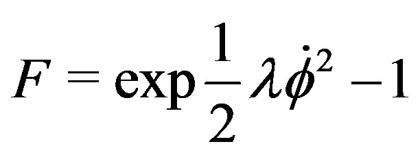 ; then we otain
 (8)
(8)
where we derive equations
 (9)
(9)
 (10)
(10)
and
 (11)
(11)
with ,
, . Note that we use the metric
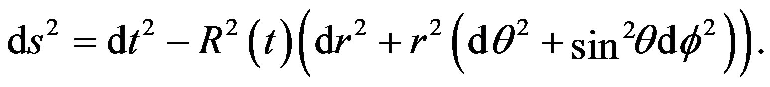 (12)
(12)
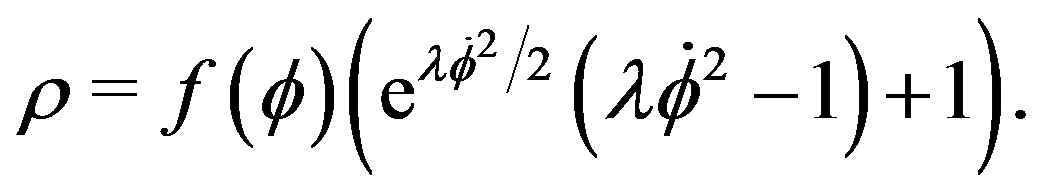
1) If we consider the parameter  very small, we can do a limited developpement of the harmonic function, the physical quantities known, the energy and the pressure can be written
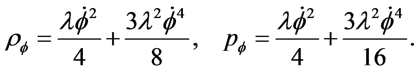 (13)
(13)
•  negative, the two physical quantities are negative; It is not physically.
•  positive, they are all positive and we obtain
 , acceptable only near the origin
 .
.
2) If  does’t allow developpment and is positive then the two physical quantities are positive and grows as an exponentially function when the Hubble constant grows.
3) If  does’t allow developpment and is negative, then we can pose
  to obtain
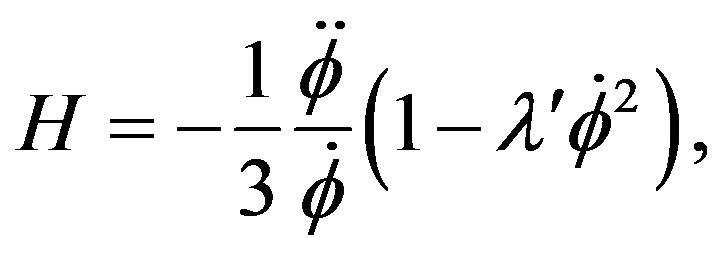 (14)
(14)
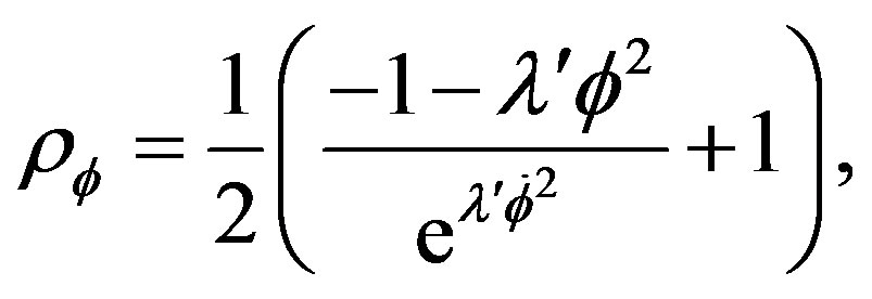 (15)
(15)
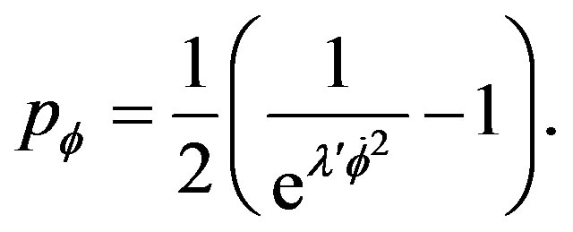 (16)
(16)
If ,
,  grows when
  and
and  decrease to zero.
 , if
, if  grows,
  decreases to
  when
when  to
to . Eliminating
  in the expression of
  and
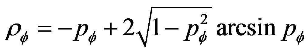
and  we get the equation of state
 (17)
(17)
By using the result of the previous section, we can first, say that there are inflation points: the point  corresponding to
  and the point
  corresponding to very large values of
 , but now this model have no point of exponential inflation model because the point
  is never attained.
2.2. Kinetical Inflation and Trigonometric Function
We consider in the action (4) the bacground matter lagrangian  negligeable, the cosmological constant equal to 0 and
 (18)
(18)
The variation of the action with respect to  gives:
 (19)
(19)
The cosmological equations come from of the variation of the action with respect to the metric
 (20)
(20)
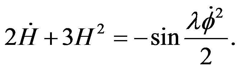 (21)
(21)
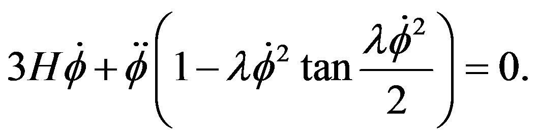
Let us derive Equation (19) and insert it into (21), then we obtain the third order differential equation:
 (22)
(22)
Let us define  and
and , then this differential equation can be written as the following system
 (23)
(23)
The state equation of this field can be written
 (24)
(24)
where  and
and 
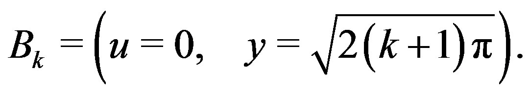
The system (23) is a dynamical system with fixed points
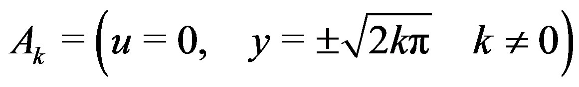 and
and
-points 
The egeinvalues equation can be written as
 .
.
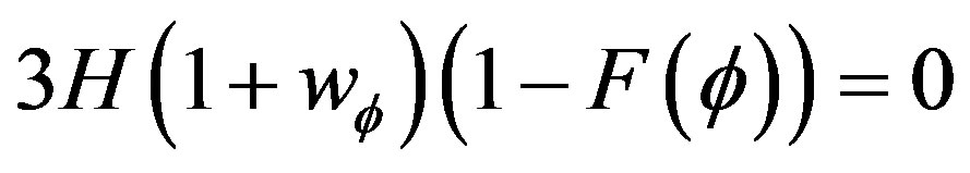
But from (20), we must have
so  must be even; and the egeinvalues can be written as:
  These points are instable fixed points. At these points,
  and the cosmological Equations (20) and (21) become:
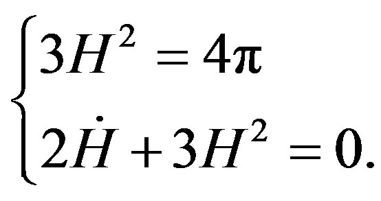 (25)
(25)
It follows that,  is negative, and
  decreases. Let us look now at the behaviour near the points
  where
where ,
,  very small. The system (23) becomes
 (26)
(26)
from where we deduce
 (27)
(27)
-points 
By the same says that the points , we find that the acceptable values of
  are old. The egeinvalues read
 .These points are stable. Near these points:
with  very small, the system (23) leads to
 (28)
(28)
So here, ; which implies
  and
and . The points
  correspond then to exponential inflation points. At these points
 . By the same, from the equation of state (24) when
 , we find
 . The points
  crrespond to a negative energy density, so it is not useful. The points
  corresponding to
  are acceptable only near the origin. The points
  correspond to the points of exponential inflation.
3. Kinetical Quintessence
Starting from , we look at the solutions of the cosmological which gives
  constant. These are the tracking solution [11]. For
  which can be written in the form
 , one poses
  an look at the solutions for which
  because in this case,
 (29)
(29)
It is the kinetical quintessence. It is shown that the tracking behaviour arise in the following case [12]
1)  and
and 
2)  and
and 
3)  and
and 
Let us look now at cases where  is a generalisation of exponentially harmonic function.
3.1. 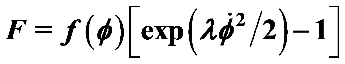
The physical quantities  and
and  can be written
 (30)
(30)
 (31)
(31)
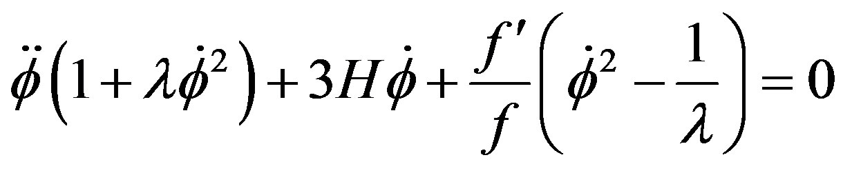
The field equation read
 (32)
(32)
We now look at the solutions which leave  as constant function of
 .
.
 (33)
(33)
 constant imply
 . With the assumption
The Hubble constant can be written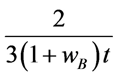 . Putting of this value in the conserved equation of the energymomentum tensor we get a function
  and the field equation becomes:
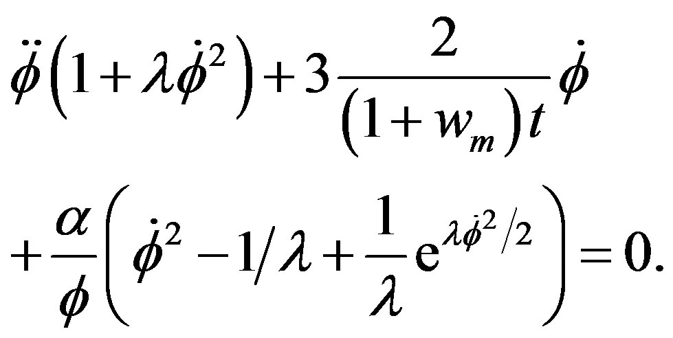 (34)
(34)
In order to eliminate t, we do the following change of variable 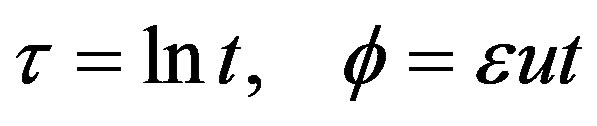 where
where  is the solution of
 (35)
(35)
Whith the condition  constant and
  constant, we can think at the tracking solutions. Here
 (36)
(36)
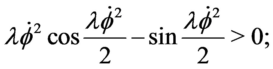
so Equation (35) has other solution than the origin if  is positive. Two cases are possible:
1) ,
, . We deduce that there are tracking solutions. Let us note that here
  is exclude.
2) , but
, but  does not verify the necessary condition. There is no tracking solutions. (34). Which the change of variables this can be read
 (37)
(37)
 (38)
(38)
The search of the fixed points of this system leads to the equation.
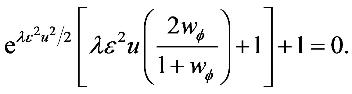 (39)
(39)
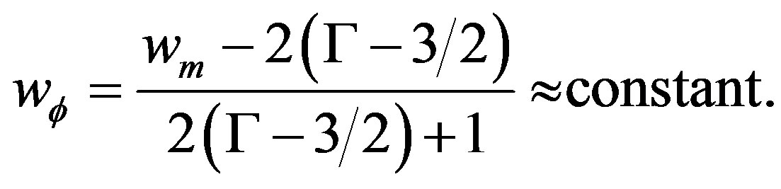
In conclusion, this form of yields have tracking solutions and these solutions are those which are acceptable to built the quintessence models ( ).
).
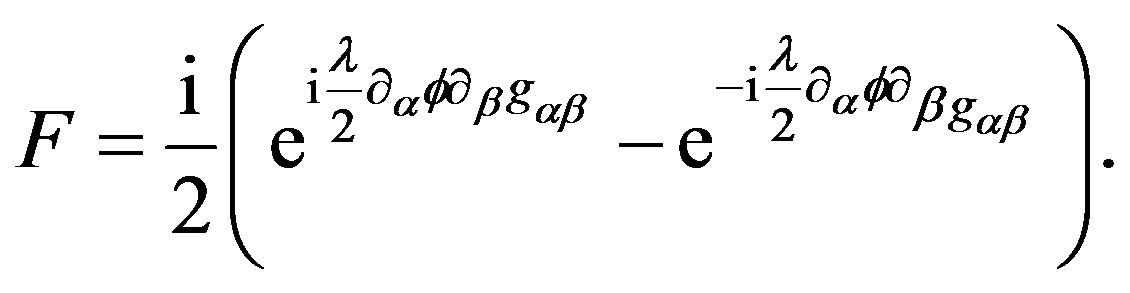
3.2. 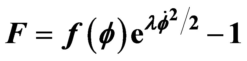
In this case the field equation take the form
 (40)
(40)
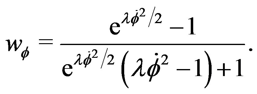
when the equation of state read
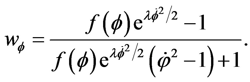 (41)
(41)
The condition  constant, imply
  and
and  are all constant. More precisely
  and
and . With the assumption
 , the conserved equation of matter leads to
 (42)
(42)
and so  if
if  Hence we can not use this condition here. But we can search the function
  for which the equation of state
  varie weakly. For that, we need a relation between
  and its derivative; what we do not find yet. However if we known the potentiel we can look at the behaviour for other quantities by the study of the following dynamical system
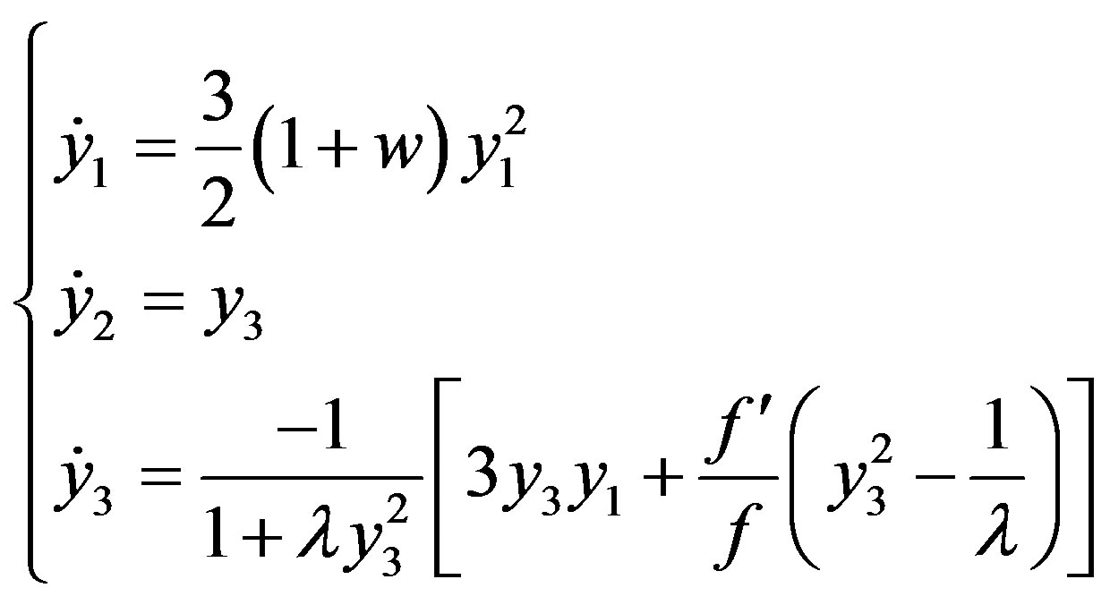 (43)
(43)
where ,
,  and
and 
4. Conclusion
Begun, there is just a few years, the use of lagrangians, not canonical, scalar fields for the description of the universe, continues to spread. It can avoid us the problems connected to the choice of the potential of the field , determining for the expected results. The problem of coincidence, however house. With the usual scalar fields, P. Steinhardt and his associates [5] were able to deduct equations of the field, the function
  which allows without an indepth study of knowledge if a model can allow to avoid the problem of coincidence by means of fields “trackers”. T. Chiba made the same thing (matter) with the lagrangians of the field of the shape
 . With the lagrangians of field exponential of the shape
  an independent relation was not able to be still found. We continue to look for a relation with the lagrangian of the shape
 .
.
REFERENCES
- P. Binétruy, “Cosmological Constant vs Quintessence,” International Journal of Theoretical Physics, Vol. 39, No. 7, 2000, pp.1859-1875. doi:10.1023/A:1003697832568
- J. P. Ostricker and P. J. Steinhard, “The Standard Cosmological Model,” Nature, Vol. 377, 1195, pp. 600-602.
- M. S. Turner, G. Steingman and L, Krauss, “The Cosmological Constant,” Physical Review Letters, Vol. 52, No. 23, 1984, pp. 2090-2093. doi:10.1103/PhysRevLett.52.2090
- P. Steinhardt, “Critical Problems in Physics,” Princeton University Press, Princeton, 1997.
- P. Steinhardt, L. Wang and I. Zlatev, “Cosmological Tracking Solution,” Physical Review D, Vol. 59, No. 12, 1999, pp. 123504-123611. doi:10.1103/PhysRevD.59.123504
- C. Armendariz-Picon, T. Darmour and V. Mukanov, “K-Inflation,” Physics Letters B, Vol. 458, 1999, pp. 209-218. doi:10.1016/S0370-2693(99)00603-6
- M. Ara, “Geometry of F-harmonic,” Kodai Mathematical Journal, Vol. 22, No. 2, 1999, pp. 243-263. doi:10.2996/kmj/1138044045
- M. Ara, “Mathematics Subject Classification,” Primary 58E20, 1991.
- M. Ara, “Mathematics Subject Classification”, Primary 58E05, 1991.
- M. Ara, “Stability of F-Harmonic Maps into Pinched Manifold,” Hiroshima Mathematical Journal, Vol. 31, No. 1, 2001, pp. 171-181.
- T. Chiba, T. Okabe and M. Yamaguchi, “Kinetical Driven Quintessence,” Physical Review D, Vol. 62, No. 2, 2000, pp. 023511-023519. doi:10.1103/PhysRevD.62.023511
- T. Chiba, “Tracking Kinetically Quintessence,” Physical Review D, Vol. 66, No. 6, 2002, pp. 063514-0635521. doi:10.1103/PhysRevD.66.063514