Journal of Modern Physics
Vol.3 No.3(2012), Article ID:18198,22 pages DOI:10.4236/jmp.2012.33033
Analysis of the Spectral Line Emissions of the Hydrogen Atom with Paraquantum Logic
1Group of Applied Paraconsistent Logic, Santa Cecília University, Santos, Brazil
2Institute for Advanced Studies, The University of São Paulo Cidade Universitária, São Paulo, Brazil
Email: inacio@unisanta.br
Received January 12, 2012; revised February 17, 2012; accepted February 28, 2012
Keywords: Paraconsistent Logic; Paraquantum Logic; Classical Physic; Relativity Theory; Quantum Mechanics
ABSTRACT
In this work we presented a study of the obtaining of the spectral line emissions of the hydrogen atom using equations that are originated from the foundations of the Paraquantum Logic (PQL). Based on a class of logics called Paraconsistent Logics with annotation of two values (PAL2v), PQL performs a logical treatment on signals obtained by measurements on physical quantities which are considered Observable Variables in the physical world. In the process of application of the PQL the obtained values are transformed in Evidence Degrees and represented on a Lattice of four Vertices where special equations transform these degrees into Paraquantum logical states ψ which propagate. This allows creating Paraquantum logical models of physical systems of the real world. Using the Paraquantum equations, we investigated the hydrogen atom spectrum and his main series known. We performed a numerical comparative study that applies the Paraquantum Logical Model to calculate the wavelengths values. The values of wavelengths obtained by the Paraquantum Equations are compared by the results found by the Rydberg formula and are verified that the series of the spectral line emissions of the hydrogen atom can be identified with the representative Lattices of the Paraquantum Logic. Through the application of the Paraquantum equations it was found a numeric value relates the layers of Paraquantum model of the Hydrogen atom. This value represents a constant that relates the Lattices that compose the Paraquantum universe, and it was denominated Paraquantum Structure Constant, whose symbol is αψ. The obtained results of the comparison demonstrate that the Paraquantum Logic comes with good possibilities of being the ideal logic to model our physical reality.
1. Introduction
A Paraconsistent Logic is a non-classical logic which revokes the principle of non-Contradiction and admits the treatment of contradictory information in its theoretical structure [1,2].
The real applications of the Paraconsistent Logic (PL) in programming of computation systems began with an interpretative form that it used annotations, and, for that reason, the PL passed to be denominated of Paraconsistent Annotated Logic (PAL). The foundational principles of the Paraconsistent Annotated Logic can be seen with details in [1] and [3,4].
1.1. Paraconsistent Annotated Logic with Annotation of Two Values (PAL2v)
The Paraconsistent Annotated Logics with annotation of two values (PAL2v) is a class of Paraconsistent Logics particularly represented through a Lattice of four vertices and from its foundations the Paraquantum Logics PQL was created. According to [4,5] we can obtain through the PAL2v a representation of how the annotations or evidences express the knowledge about a certain proposition P. This is done through a lattice on the real plane with pairs (m, λ) which are the annotations. In this representation an operator is fixed: ~:|t| ® |t| where t = {(m, λ) |m, λ Î [0, 1] Ì Â}. The extreme logical Paraconsistent states which are the four vertices of the lattice with Favorable Degree of evidence μ and Unfavorable Degree of evidence λ as seen in Figure 1. With P(μ, λ) we read them in the following way:
PT = P(1, 1) → The annotation (m, l) = (1, 1) assigns intuitive reading that P is inconsistent.
Pt = P(1, 0) → The annotation (m, l) = (1, 0) assigns intuitive reading that P is true.
PF = P(0, 1) → The annotation (m, l) = (0, 1) assigns intuitive reading that P is false.
P^= P(0, 0) → The annotation (m, l) = (0, 0) assigns intuitive reading that P is Indeterminate.
In the internal point of the lattice which is equidistant
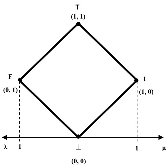
Figure 1. Lattice of four vertexes and representation of the extreme logical Paraconsistent states.
from all four vertices, we have the following interpretation: PI = P(0.5, 0.5) → The annotation (m, l) = (0.5, 0.5) assigns intuitive reading that P is undefined.
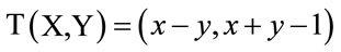
As it can be seen in the study of the PAL presented in [5] with the values of x and y that vary between 0 and 1 and being considered in an Unitary Square on the Cartesian Plane (USCP), we can get linear transformations for a Lattice k of analogous values to the associated Lattice τ of the PAL2v. We obtain the following final transformation:
 (1)
(1)
According to the language of the PAL2v [5] we have:
x = m → is the Favorable evidence Degree;
y = λ → is the Unfavorable evidence Degree.
The first coordinate of the transformation (1) is called Certainty Degree DC. So, the Certainty Degree is obtained by:
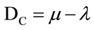 (2)
(2)
The second coordinate of the transformation (1) is called Contradiction Degree Dct. So, the Contradiction Degree is obtained by:
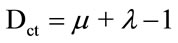 (3)
(3)
The second coordinate is a real number in the closed interval [–1,+1]. The y-axis is called “axis of the contradiction degrees”. From (2), (3) and (1) we can represent a Paraconsistent logical state eτ into Lattice τ of the PAL2v [5], such that:
 (5)
(5)
where eτ is the Paraconsistent logical state.
DC is the Certainty Degree obtained from (2);
Dct is the Contradiction Degree obtained from (3).
The Paraconsistent logical state eτ can be anywhere in the lattice τ, and a real Certainty Degree DCR can be obtained as follows. For  we compute:
 (6)
(6)
For  we compute:
 (7)
(7)
where  and
and 
For DC = 0 we consider the undefined Paraconsistent logical state with: DCR = 0.
1.2. The Paraquantum Logic PQL
In recent applications of the PAL2v (see [6,7]) there was the need of including restrictions in its algorithms. The restrictions were necessary because under certain conditions the results obtained from the model changed through leaps or unexpected variations. Later, it was seen in research based on PAL2v models that the application of its foundations offered results strongly connected to the ones found in modeling of phenomena studied in quantum mechanics [7,8]. Following this idea, the special features of the PAL2v are applied in the form of variations of values from the concepts of the Paraquantum Logics PQL (see [9,10]).
1.3. The Paraquantum Function ψ(PQ) and the Paraquantum Logical State ψ
For each measurement performed in the physical world of μ and λ, we obtain a unique duple  which represents a unique Paraquantum logical state ψ which is a point of the lattice of the PQL. Therefore, a Paraquantum function y(Py) is defined as the Paraquantum logical state y (see [11,12]):
 (8)
(8)
where m, λ Î [0,1] Ì Â.
On the vertical axis of contradictory degrees, the two extreme real Paraquantum logical states are (see [10]):
1) The contradictory extreme Paraquantum logical state which represents Inconsistency T:
ψT
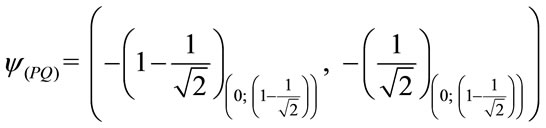
2) The contradictory extreme Paraquantum logical state which represents Undetermination ^:
On the horizontal axis of certainty degrees, the two extreme real Paraquantum logical states are:
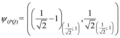
1) The real extreme Paraquantum logical state which represents Veracity t:
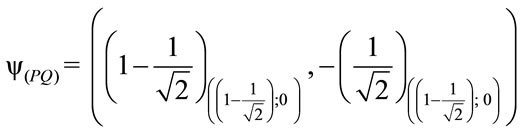
2) The real extreme Paraquantum logical state which represents Falsity F:
 .
.
1.4. The Vector of State P(ψ)
A Vector of State P(ψ) will have origin in one of the two vertexes that compose the horizontal axis of the certainty degrees and its extremity will be in the point formed for the pair indicated by the Paraquantum function [11,12]:
If the Certainty Degree is negative (DC < 0), then the Vector of State P(ψ) will be on the lattice vertex which is the extreme Paraquantum logical state False: ψF = (–1, 0).
If the Certainty Degree is positive (DC > 0), then the Vector of State P(ψ) will be on the lattice vertex which is the extreme Paraquantum logical state True: ψt = (1, 0). If the certainty degree is nil (DC = 0), then there is an undefined Paraquantum logical state ψI = (0.5, 0.5).
The Vector of State P(ψ) will always be the vector addition of its two component vectors:
XC Vector with same direction as the axis of the certainty degrees (horizontal) whose module is the complement of the intensity of the certainty degree: 
Yct Vector with same direction as the axis of the contradiction degrees (vertical) whose module is the contradiction degree: 
Given a current Paraquantum logical state ψcur defined by the duple  then we compute the module of a Vector of State P(ψ) as follows:
 (9)
(9)
where DC = Certainty Degree computed by (2);
Dct = Contradiction Degree computed by (3).
Using (9) which is for computing the module of a Vector of State P(ψ), we have:
1) For DC > 0 the real Certainty Degree is computed by:
 (10)
(10)
where:
DCψR = real Certainty Degree;
DC = Certainty Degree computed by (2);
Dct = Contradiction Degree computed by (3).
2) For DC < 0, the real Certainty Degree is computed by:
 (11)
(11)
where:
DCψR = real Certainty Degree;
DC = Certainty Degree computed by (2);
Dct = Contradiction Degree computed by (3).
3) For DC = 0, then the real Certainty Degree is nil.
The inclination angle ay of the Vector of State which is the angle formed by the Vector of State P(y) and the x-axis of the certainty degrees is computed by:
 (12)
(12)
1.5. Uncertainty Paraquantum Region
The propagation of the superposed Paraquantum logical states ysup through the lattice of the PQL happens due to the continuous measurements performed on the observable variables in the physical world [10,11]. When the module of the Vector of State MP(ψ) = 1, this vector will represent the maximal fundamental superposed Paraquantum logical states ψsupfmax which has real certainty degrees zero. The maximum Contradiction Degree for this condition is when the Vector of State P(ψ) forms an angle of 45˚ with the horizontal axis of certainty degrees. Therefore, given that the inclination angle of the Vector of State is  = 45˚ then the maximum Contradiction Degree for this condition is computed by:
We observe that this same condition is found when the Vector of State has inclination angle , or still, with origin in the extreme Vertex representative of the extreme False Paraquantum logical state. In that extreme contradictory situation the module of the Vector of State MP(ψ) will have his maximum value of:
 .
.
The unbalanced contradictory Paraquantum logical state ψctru is the one located on the lattice of states of the PQL where there is a condition of opposite signs between the Certainty Degree (DC) and the real Certainty Degree (DCψR). The Paraquantum logical states into limits of the Region of Uncertainty are identified with Factors of maximum limitation of transition [11]. With Paraquantum Logic state  these factors are:
1. The factor of Paraquantum limitation False/inconsistent—hQyFT.
 º hQyFT
2. The factor of Paraquantum limitation True/inconsistent—hQytT.
 º hQytT
3. The factor of Paraquantum limitation False/undetermined—hQyF^.
 º hQyF^
4. The factor of Paraquantum limitation True/undetermined—hQyt^.
 º hQyt^
All the Superposed Paraquantum logical states ysup to these and that they will have variation of the inclination angle until null degree delimit the Region of Uncertainty of the Lattice of PQL.
1.6. The Paraquantum Factor of Quantization hψ
When the superposed Paraquantum logical state ysup propagates on the lattice of the PQL a value of quantization for each equilibrium point is established. This point is the value of the contradiction degree of the Paraquantum logical state of quantization yhy [11] such that:
 (13)
(13)
where hy is the Paraquantum Factor of quantization.
The factor hy quantifies the levels of energy through the equilibrium points where the Paraquantum logical state of quantization yhy, defined by the limits of propagation throughout the uncertainty of the PQL, is located. Figure 2 shows the interconnections between the factors and its characteristics, in which they delimit the Region of Uncertainty in the Lattice of PQL.
1.7. The Paraquantum Factor of Quantization and Paraquantum Leap
In a process of propagation of Paraquantum logical state y, we have in the instant that the superposed Paraquantum logical state ysup reaches the representative points of the limiting factors of the uncertainty region of the PQL, the Certainty Degree (DC) remains zero but the real Certainty Degree (DCyR) will be increased or decreased from zero and this difference corresponds to the effect called of the Paraquantum Leap [11]. Concerning the action of the Paraquantum Factor of quantization hψ on the PQL Fundamental Lattice, we must also consider the effect of the Paraquantum Leap that produces quantities that will be either added or subtracted. So, the Paraquantum Factor of quantization in its complete or total form which acts on the quantities is:
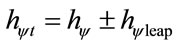 (14)
(14)
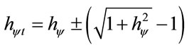 (15)
(15)
Figure 3 shows the effect of the Paraquantum Leap in the quantization of values when the Superposed Paraquantum Logical states ysup reach the point where the Paraquantum Logical state of Quantization ψhψ on the PQL Lattice.
Being: 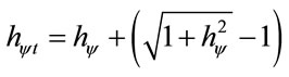 the total Paraquantum Factor of quantization at the time of arrival of the Superposed Paraquantum Logical state ψsup at the point where the Paraquantum Logical state of Quantization ψhψ is located.
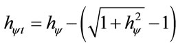 is the total Paraquantum Factor of quantization at the departure of the Superposed Paraquantum Logical state ψsup at the point where the Paraquantum Logical state of Quantization ψhψ is located. Around the Paraquantum logical state of pure Indefinition yIP, the variation of values inside the limits can be expressed by [11,12]:
 (16)
(16)
These logical states establish connection in the point where the logical Paraquantum state of quantization yhy is situated.
At the instant that the superposed Paraquantum logical states ysup visit the Paraquantum logical state of quantization yhy, the real Certainty Degree will have variations of the form:
 (17)
(17)
When the Paraquantum logical states ysup visit the Paraquantum state of quantization yhy established by the Paraquantum Factor of quantization hy, the Paraquantum Leap happens (see [11,12]).
1.8. The Fundamental Lattice of the PQL
The contraction of the Fundamental Lattice points out that the Paraquantum Logical state ψ is an infinitely contracted Fundamental Lattice and has, through the Paraquantum Factor of quantization hψ, all features of the PQL Fundamental Lattice (see [11,12]).
The quantitative analysis on the PQL Lattice defines a quantitative value QValor of any physical quantity, which can be represented on the horizontal axis of the certainty
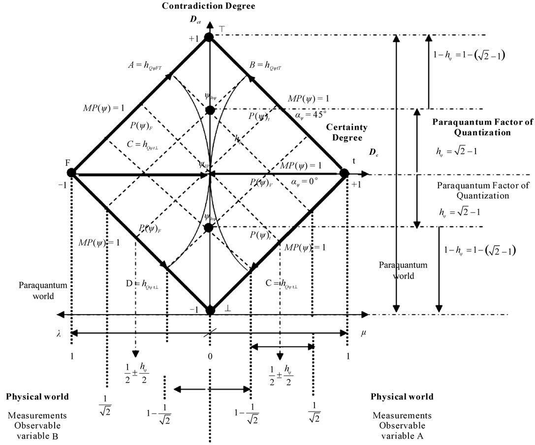
Figure 2. The Paraquantum factor of quantization hy related to the evidence degrees obtained in the measurements of the observable variables in the physical world.
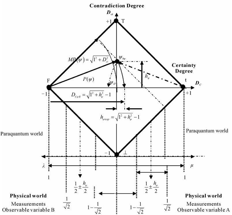
Figure 3. The Paraquantum factor of quantization on the Paraquantum logical state of quantization yhy due to Paraquantum leap.
Degrees and on the vertical axis of the contradiction degrees of the PQL Lattice. Since the maximum value is normalized on the PQL Fundamental Lattice, considering the Paraquantum factor of quantization only, we can write:
 (18)
(18)
Doing so, the unitary value of the quantization is equivalent to a Paraquantum quantization represented in the Paraquantum Logical state ψhψ added to the value of its complement. We have:
 (19)
(19)
where  is the value of the total amount represented on the unitary axis of the PQL Fundamental Lattice.
Equation (19) shows that the maximum amount of any quantity in the physical environment is composed by two quantized fractions where: one is determined on the Paraquantum Logical state of Quantization ψhψ by the Paraquantum Factor of quantization hψ and the other is determined by its complement (1 – hψ).
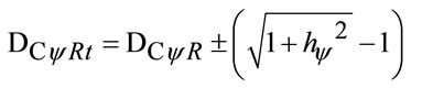
Since it is a value related to the Paraquantum Logical Model, this radius of the horizontal propagation is determined through a Paraquantum quantity computed by:
 (20)
(20)
So, for the Energy, the equation is:
 (21)
(21)
We can define the equation of the energy levels such that:
 (22)
(22)
where  is the total Energy which can be transformed through propagation.
 is the maximum Energy on level N of the transition frequency N is the transition frequency or number of times of application of the Paraquantum Factor of quantization.
We verify that, in the same way for quantities, the energy is quantized through the equilibrium point established by the Paraquantum Logical state of Quantization ψPψ.
2. Paraquantum Logic and Levels of Energy in the Bohr Model
A Paraquantum Logical model where the Superposed Paraquantum Lattices are related in both the physical and Paraquantum environments and produce levels of energy which will be used to analyze the Hydrogen atom.
Based on Equation (22) the equation of the quantities of Energy, for the Bohr’s model on the Hydrogen atom, can be written as follows:
 (23)
(23)
where: hψ is the Paraquantum Factor of quantization .
.
 is the total Energy that can be transformed through propagation, therefore through the orbit of the electron in the Hydrogen atom.
 is the maximum energy on the level N of transition frequency or in the current state of excitation of the electron.
N is the transition frequency or number of times of application of the Paraquantum Factor of quantization.
The value of the quantity of Energy of Propagation quantized, when considered in its static form, therefore, without considering the effect of the Paraquantum Leap, is computed by:
 (24)
(24)
where hψ is the Paraquantum Factor of quantization..
 is the Energy transformed in the propagation of the Paraquantum Logical state of the extreme Vertex False until it reaches the point where the Paraquantum Logical state of Quantization ψhψ is located.
 is the maximum Energy on the level N of the transition frequency or on the current state of excitation of the electron.
Since the process of transformation of energy is dynamical, we must consider the effects of Paraquantum Leaps on the Paraquantum Logical Model. So, the Inertial or Irradiating Energy is expressed by:
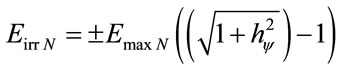 (25)
(25)
If Bohr’s Model [13,14] is used in the paraquantum analysis, the electron will be considered a Paraquantum Logical state ψ–e that propagates orbiting the logical state proton ψ+Z located on the Paraquantum Logical state Undefined ψI. So, the positive or negative sign of the equation (25) indicates if the analysis is at the arrival or at the departure of the electron at the equilibrium point where the Paraquantum Logical state of Quantization ψhψ is located. Since the electron, in the Model of Hydrogen Atom, reaches the excitation level at the arrival at the equilibrium point, then the sign will positive at the instant of the analysis, only. So, the total energy transformed at the equilibrium point of the Lattice of the PQL is computed by:
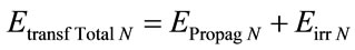 (26)
(26)
So, Equation (23) is rewritten as follows:
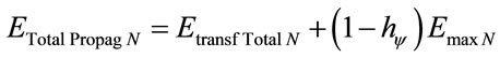 (27)
(27)
or as follows:
 (28)
(28)
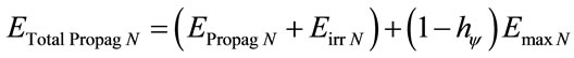
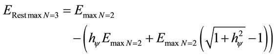
Or, in a more complete way, as follows:
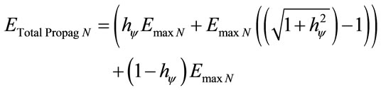 (29)
(29)
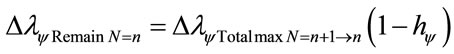
The second term of Equation (29) is the complemented value which represents the remaining maximum energy, therefore, it is that amount of energy capable of still being transformed in order to increase the excitation level of the electron. So, for each new excitation level of the electron, the remaining energy ERestmax is the one which outcomes the value which will be represented on the vertical and horizontal axis of the Lattice of the PQL.
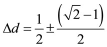
For a static analysis, we have:
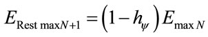 (30)
(30)
or
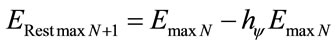 (31)
(31)
From (31) the energy variation value is expressed by:
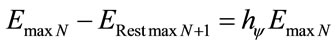 (32)
(32)
Therefore, the remaining maximum Energy in the atom model depends on the excitation level of the electron.
When the analysis process is considered dynamical, we must take the effect of the Paraquantum Leap into account and determine the Remaining maximum Energy adding the Inertial or Irradiating Energy. So, Equation (31) in its complete form is:
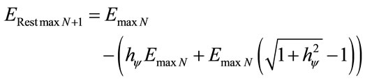 (33)
(33)
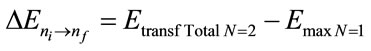
And the energy transformed value between the Fundamental level n = 1 and the level N = n is:
 (34)
(34)
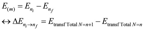
For variation of Energy between two levels:
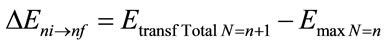 (35)
(35)
Figure 4 shows a Paraquantum Logical model where the physical and Paraquantum environments produce levels of energy for analyze of the Hydrogen atom.
Analyses of the Hydrogen Atom in Lattice of the PQL
Following the application methods of the PQL [11,12] we will make a study that represents the Hydrogen atom on the Lattice of the PQL considering the results of the postulates of Bohr with the correlation features of the effects of propagation of the Paraquantum Logical states ψ and the bounding Factors of the Uncertainty Region of the PQL. So, the electron is considered a Superposed Paraquantum Logical state ψsup represented by ψ–el that propagates through the Fundamental Lattice of the PQL from the Vertex which represents the extreme Paraquantum Logical State False. The propagation will be expressed through energy quantization determined by the Paraquan tum Factor of quantization hψ considering the Paraquantum Leaps through the variations on the value of the Real Certainty Degree that identifies the appearing of inertial or irradiating energy.
In the physical world, the insertion of energy into the atom causes disequilibrium and, if this disequilibrium is enough, it causes the electron to leave its fundamental state n = 1 and it makes the electron to reach another state of excitation. On the Fundamental Lattice of the PQL that represents the Hydrogen Atom, the Paraquantum logical state ψ–erel of the electron when propagating will transform the energy represented on the axis of the Certainty and Contradiction degrees and, for this, moves diagonally to one of the extreme Vertices of contradiction. When the Electron receives energy enough to reach another exciting state for n = 2, it means that the potential energy represented on the horizontal axis of the certainty degrees (EnDC) of the initial conditions is transformed in kinetic energy represented on the horizontal axis of the certainty degrees (EnDct) and reached enough to take it up, through two transitions to the excited level at the point where the Paraquantum Logical state of Quantization ψhψ is located. Figure 5 shows the propagation of the electron around the proton on the fundamental state n = 1.
This change of the electron from a state to another is done on the Paraquantum Logical model through the characteristics of the correlation that implies in considering the effects in the physical environment reflected on the paraquantum world.
3. Application of the Paraquantum Logic (PQL) in the Atom of Hydrogen
The correlation characteristics of the Relativistic Paraquantum Lattice and the transience property of the Superposed Paraquantum Logical states ψsup which propagate on the Fundamental Lattice of the PQL provide us with several conditions to make a comparative study of the Hydrogen atom using Bohr’s model [14,15]. This study can be made directly with the energy levels of the Paraquantum correlation states through the equation that deals with quantities. So, each time that there is an increase of Energy defined by the Paraquantum Factor of quantization hψ, there will be two transitions of the electron that will make it perform an orbit of a level of excited state in the Hydrogen atom. At the end of these two transitions of the electron, represented by the Paraquan-
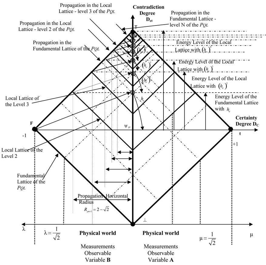
Figure 4. Model of the superposed local fundamental lattices where we can represent systems of energizing levels through the fundamental lattice.
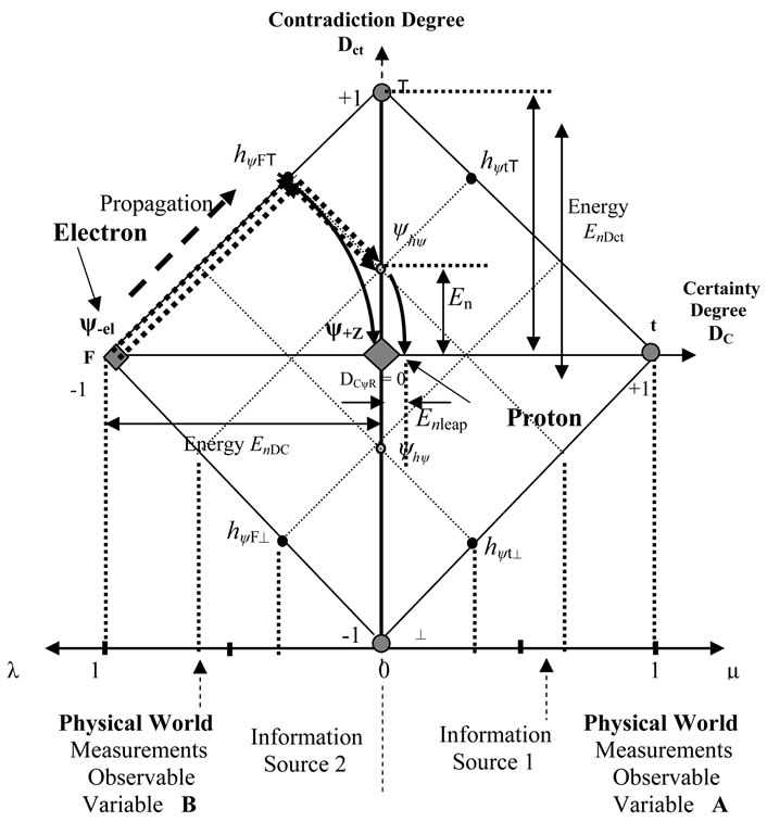
Figure 5. First propagation of the Paraquantum logical state ψ–el which represents the electron at the fundamental state n = 1 passes by the Paraquantum logical state of quantization ψhψ with the energy being quantized by the Paraquantum factor of quantization hψ.
tum Logical state ψ–el, it will be on the equilibrium point of the Paraquantum Logical state of Quantization ψhψ. The energy on this point is determined by the addition of the energy transformed in the propagation Etporp with the Inertial of Irradiant Eirr which appears due to the Paraquantum Leaps [11,12]. In 1913, Niels Bohr proposed a model for the Hydrogen atom. According to the Bohr’s Postulate [15], the angular momentum of the electron is quantized and it is an integer number (n): . Comparing to its corresponding in the classical mechanics (
 ), we can find and define the value of r in function of n. So, we have:
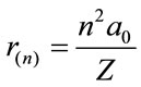 (36)
(36)
where a0 is the constant called radius of Bohr. Because of that we have that the radius of the stationary states are quantized with a value defined by the previous equation in function of a0 with value of n > 0. By determining the expression of rn, we can find the expression of total Energy (En of the electron) which is also quantized, that is, the stationary states correspond to specific values of certain amount of energy [15]. The equation of total Energy is expressed by:
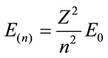 (37)
(37)
with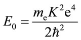 .
.
We verify in this equation that En appears with a multiple of E0, whose value can be found and corresponds to 2.18 × 10⁻¹⁸ J or 13.6 eV.
According to Bohr’s postulate, the energy for an electronic transition, according to the set of allowed energies Em from position ni to position nf, is defined by:
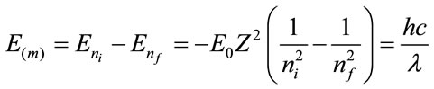 (38)
(38)
This value is the inverse of the wavelength and Bohr compared it with the Rydberg-Ritz Formula, obtaining the theoretical value of the Rydberg’s constant.
3.1. Values of Energy Quantities on Levels of Energy through the Paraquantum Equations
Through the Paraquantum equations and the interpretation on the Lattice of the PQL, from where we obtain the energy levels with consecutive applications of the correlation factors, we can compute the values found on Bohr’s model for the Hydrogen atom.
• For the fundamental state n = 1
Initially, we have, on the fundamental state, the value that generates the Fundamental Lattice of the PQL for the Paraquantum Logical Model as being the value of Energy obtained by the Bohr’s equations such that the Total Energy of the electron is: .
.
Using the value of the Energy obtained by the Bohr’s equations we can compute the Propagation Energy of the electron when it propagates through the Fundamental state by Equation (24).
 →
→
→
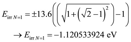
According to the Paraquantum Logical Model, the propagation of the electron is done on the edges of the Uncertainty Region of the Lattice of the PQL, so when it crosses the Vertical axis of the contradiction degrees on the point where the Paraquantum Logical state of Quantization ψhψ is located, we have the Inertial or Irradiant Energy caused by the Paraquantum Leap. The Inertial or Irradiant Energy for the Fundamental level is computed by Equation (25) such that:
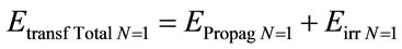
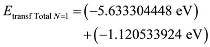
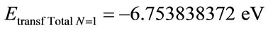
With Equation (26), the total transformed Energy for the Fundamental level is computed by:
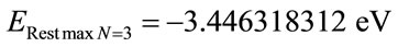
Through Equation (33) for the second level of excitation n = 2, we have the Remaining Energy to be transformed and it is computed by:

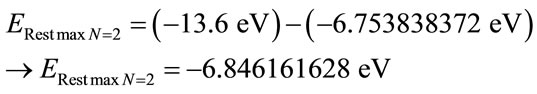
The Remaining Energy will be the Total Energy of the electron that will constitute the second Lattice of the PQL for the representation of the propagation of the electron at the excitation level n = 2.
• For the excited state n = 2
→
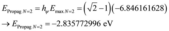
By Equation (24) we have the Propagation Energy at the second excitation state of the electron n = 2 computed by:
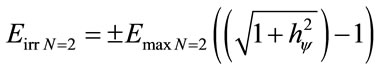
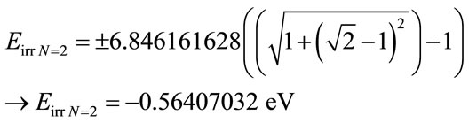
With Equation (25) the Inertial or Irradiant Energy for the level of the second excitement state of the electron n = 2 computed by:
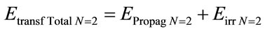
By Equation (26) the total transformed Energy to the level of the second excitement state of the electron n = 2 is computed by:

→
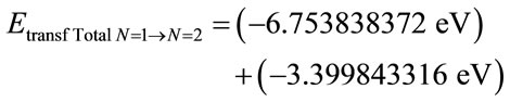
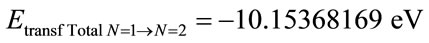
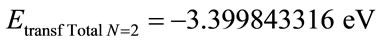
The Total transformed energy to the level of the second Excitement state of the electron n = 2 with respect to the Fundamental state is computed by Equation (34):

By Equation (33) to the second excitation level n = 2, we have the Remaining Energy to be transformed which is computed by:

→
By Equation (35) the variation Energy between two consecutive levels is:

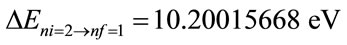
and 
With the Paraquantum equations we can calculate the variations of energy in infinites levels of the Lattice, therefore of the Paraquantum model of hydrogen atom.
The values obtained through the Paraquantum Equations (26), (34) and (35) for the Hydrogen atom model in seven energy levels:
• For Level n = 2:


• 
• For Level n = 3:

• 
• For Level n = 4:

• 
• For Level n = 5:
• 
• For Level n = 6:
• 
• For Level n = 7:
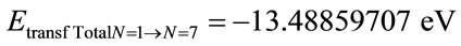
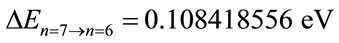
Figure 6 shows a Paraquantum Logical model with the energy values calculated by Paraquantum Equations (26) and (34) in each levels of energy of the Hydrogen atom.
3.2. The Spectrum of Radiation
Atomic spectra—which is the characteristic radiation emitted by the atoms of elements when they are heated, or submitted to electrical discharges—were studied at the end of the XIX century [13-15].
When observed with a spectroscopy, the radiation shows as a series of lines with different wave lengths, not always on a visible spectrum. Among many scientists that studied the atomic spectra, J. R. Rydberg and W. Ritz determined an empirical expression capable of compute the sequence of these lines. This expression is known as the Rydberg-Ritz formula and is given by:
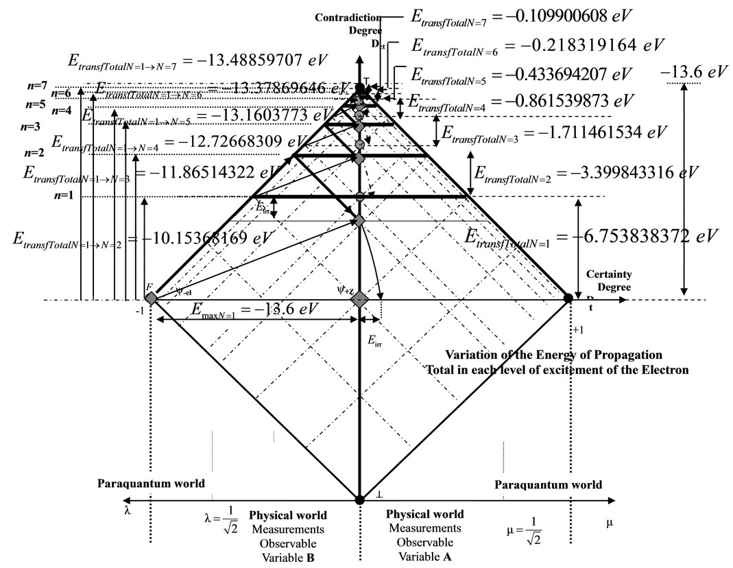
Figure 6. Paraquantum logical model with energy values of the hydrogen atom.
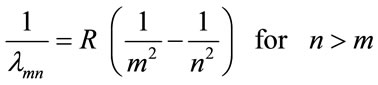 (38)
(38)
where m and n are integers and R is the Rydberg constant, with result expressed in meters.
This constant is the same for all lines of the spectrum of the same elements, varying slightly and regularly according to the elements. For Hydrogen, the value of R is 1.096776 × 10⁷ m–1 approaching a limit value of 1.097373 × 10⁷ m–1 for heavy elements [14].
This empirical expression can preview lines that are out of the range of the visible spectrum and have not been observed yet.
3.3. The Hydrogen Spectral Series
As it can be seen in [13,14] the emission spectrum of atomic hydrogen is divided into a number of spectral series, with wavelengths given by the Rydberg formula. These observed spectral lines are due to electrons moving between energy levels in the atom. When an electron jumps from a higher energy to a lower, a photon of a specific wavelength is emitted. Calculating the wavelength using the equation (38) the spectral lines are grouped into series according to n', such that:
1) Lyman series (n′ = 1)
n 2 3 4 5 6 7
λ(nm) 121.6 102.5 97.2 94.9 93.7 93.0
n 8 9 10 11 12 ∞
λ(nm) 92.6 92.3 92.1 91.9 91.11 91.15
2) Balmer series (n′ = 2)
n 3 4 5 6 7
λ(nm) 656.3 486.1 434.1 410.2 397.0
n 8 9 ∞
λ(nm) 388.9 383.5 364.2
3) Paschen series (n′ = 3)
n 4 5 6 7 8
λ(nm) 1875.1 1281.8 1093.8 1004.9 922.9
n 9 10 11 12 13 ∞
λ(nm) 954.6 901.5 886.3 875.0 866.5 820.4
4) Brackett series (n′ = 4)
n 5 6 7 8 9 ∞
λ(nm) 4050 2630 2170 1940 1820 1460
5) Pfund series (n′ = 5)
n 6 7 8 9 10 ∞
λ(nm) 7460 4650 3740 3300 3040 2280
6) Humphreys series (n′ = 6)
n 7 8 9 10 11 ∞
λ(nm) 12400 7500 5910 5130 4670 3280
3.4. Calculations of the Wavelength Values of Each One of the Six Series with Paraquantum Equations
For each series of the spectrum of the atom of Hydrogen the wavelengths can be calculated through the Paraquantum equations. The energy variation between levels of the Equation (38) 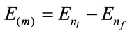 can be computed by Paraquantum Equation (34), therefore:
And considering the Equation (38) the Paraquantum wavelengths can be calculated by:
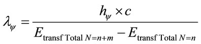 (39)
(39)
where c is the constant of the light speed in the vacuum 299,792,458 m/s and n ≥ 1.
As seen in [10,11], the value of the Paraquantum Factor of quantization hψ when expressed in the International System (SI) is: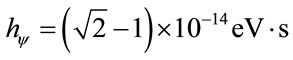 . This way, the unit of measure of the wavelength can be presented in 10–9 m (nm).
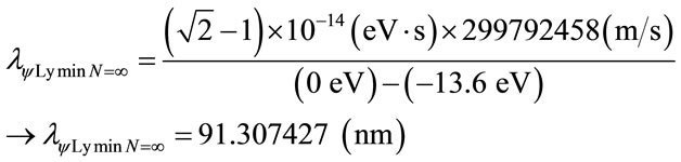
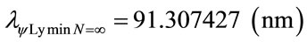
1) For the Lyman series (n′ = 1).
and 
Then from Equation (39) the maximum wavelength value is:
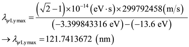
Considering the energy variation between levels computed by Equation (35) for , then for Equation (39)
 :
:  and
and 
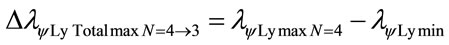
For the PQL Lattice the total maximum wavelengths values is identified with:
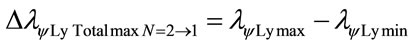

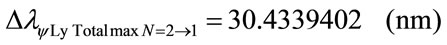
The wavelength value in the level 2 is compared with variation energy Equation (26):
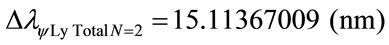
The variation of wavelength value pure for N = 2:

The variation of the Paraquantum Leap effect in the wavelength, for N = 2:
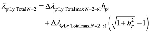
The variation of wavelength value total, which is, considering the Paraquantum Leap effect, for N = 2:


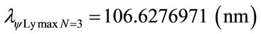
Subtracting the value of the variation for the total value is obtained the wavelength of the level 3:

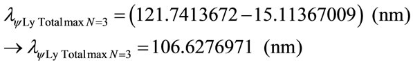
In the same way for next level n = 3:
Consider: 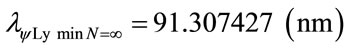
For the PQL Lattice the total maximum wavelengths values is identified with:


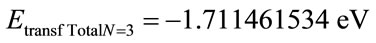
The wavelength value in the level 3 is compared with variation energy Equation (26):

The variation of wavelength value pure for N = 3:

The variation of the Paraquantum Leap effect in the wavelength, for N = 3:

The variation of wavelength value total, which is, considering the Paraquantum Leap effect, for N = 3:
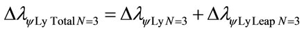

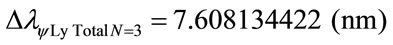
Subtracting the value of the variation for the total value is obtained the wavelength of the level 4:

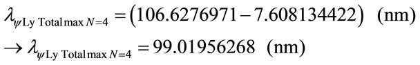
In the same way for next level n = 4:
Consider:

For the PQL Lattice the total maximum wavelengths values is identified with:

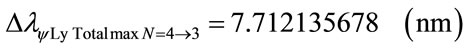
The wavelength value in the level 4 is compared with variation energy Equation (26):
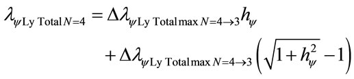
The variation of wavelength value pure for N = 4:


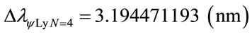
The variation of wavelength value total, which is, considering the Paraquantum Leap effect, for N = 4:


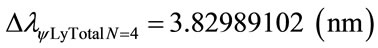
Subtracting the value of the variation for the total value is obtained the wavelength of the level 5:

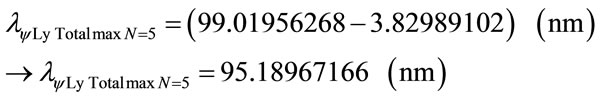
Using the same mathematical procedures with the Paraquantum equations was obtained the following wavelength values:
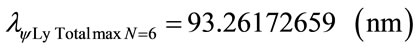
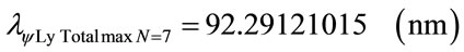
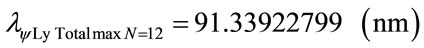
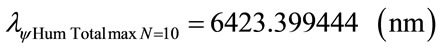
Figure 7 shows the Paraquantum wavelength values of the Lyman series in the Paraquantum Model of the Hydrogen atom (n′ = 1).
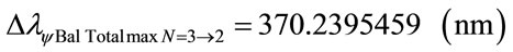
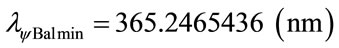
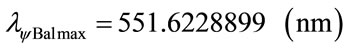
2) Using the same mathematical procedures with the Paraquantum equations for Balmer series (n′ = 2):
and 
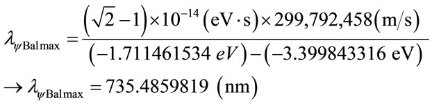
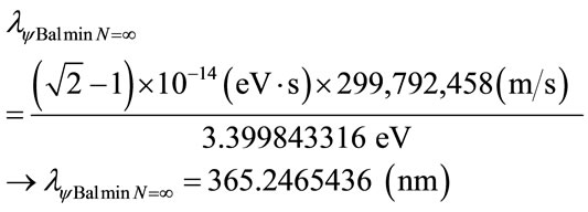
Then from Equation (39) the maximum wavelength value is:
Considering the energy variation between levels computed by Equation (35) for :
:
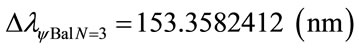
For the PQL Lattice the total maximum wavelengths values is identified with:


The wavelength value in the level 3 is compared with variation energy Equation (26):
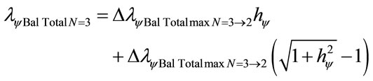
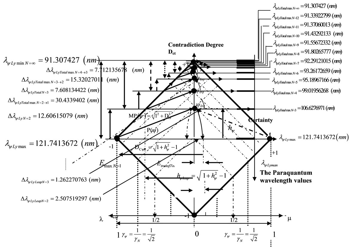
Figure 7. Representation in the lattice of the Paraquantum wavelength values for lyman series.
The variation of wavelength value pure for N = 3:


The variation of the Paraquantum Leap effect in the wavelength, for N = 3:

The variation of wavelength value total, which is, considering the Paraquantum Leap effect, for N = 3:

The wavelength of the level 4 is:
In the same way for next level n = 5:
Consider:
Using the same mathematical procedures with the Paraquantum equations was obtained the following wavelength values:
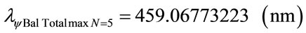
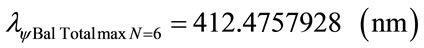
Figure 8 shows the Paraquantum wavelength values of the Balmer series (n′ = 2).
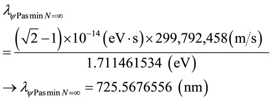
3) Using the same mathematical procedures with the Paraquantum equations for Paschen series (n′ = 3):

Then from Equation (39) the maximum wavelength value is:
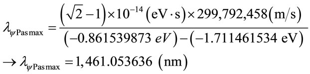
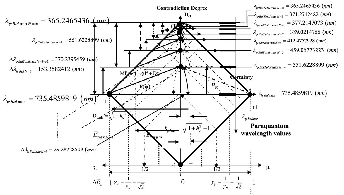
Figure 8. Representation in the lattice of the Paraquantum wavelength values of the balmer series (n′ = 2).
Considering the energy variation between levels computed by Equation (35) for :
:
For the PQL Lattice the total maximum wavelengths values is identified with:


The wavelength value in the level 4 is compared with variation energy Equation (26):

The variation of wavelength value pure for N = 4:

Considering the Paraquantum Leap effect, for N = 4:

The wavelength of the level 5 is:
In the same way for next level n = 6:
Consider:
With the Paraquantum equations was obtained the following wavelength values:


Figure 9 shows the Paraquantum wavelength values of the Paschen series (n′ = 3).
4) Using the same mathematical procedures with the Paraquantum equations for Brackett series (n′ = 4):

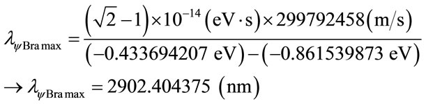
Considering the energy variation between levels computed by Equation (35) for :
:
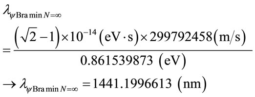
For the PQL Lattice the total maximum wavelengths values is identified with:

The wavelength value in the level 5 is compared with variation energy Equation (26):

The variation of wavelength value pure for N = 5:

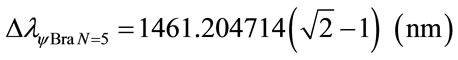
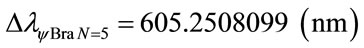
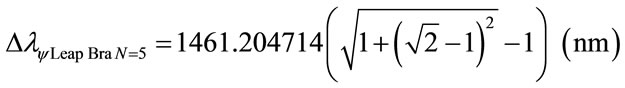
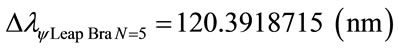
Considering the Paraquantum Leap effect, for N = 5:

The wavelength of the level 6:

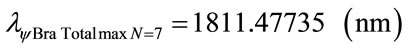
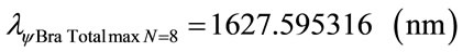
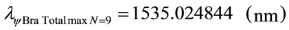
In the same way for next level n = 7:
Consider:
was obtained the following wavelength values:
5) Using the same mathematical procedures with the Paraquantum equations for Pfund series (n′ = 5):


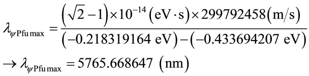
For the PQL Lattice the total maximum wavelengths values is identified with:

Compared with variation energy Equation (26):

The variation of wavelength value pure for N = 6:

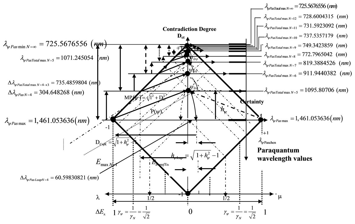
Figure 9. Representation in the lattice of the Paraquantum wavelength values of the Paschen series (n′ = 3).
Considering the Paraquantum Leap effect, for N = 6:

The wavelength of the level 7:


→
In the same way for next level n = 8:
Consider:
was obtained the following wavelength values:
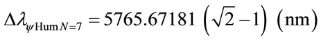
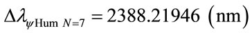
6) Using the same mathematical procedures with the Paraquantum equations for Humphreys series (n′ = 6):
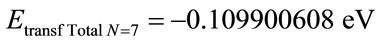
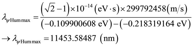
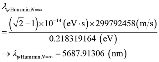
For the PQL Lattice the total maximum wavelengths values is identified with:


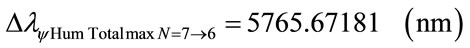
The wavelength value in the level 7 is compared with variation energy Equation (26):
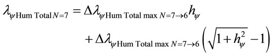
The variation of wavelength value pure for N = 7:

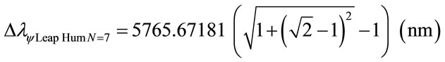
Considering the Paraquantum Leap effect, for N = 6:

The wavelength of the level 8:

In the same way for next level n = 9:
Consider:
was obtained the following wavelength values:


The representations of each one of the series Brackett, Pfund and Humphreys are identical shown them in the Figures 8-10.
3.5. The Study of the Series in the Paraquantum Universe
The values of the wavelengths of the series found through
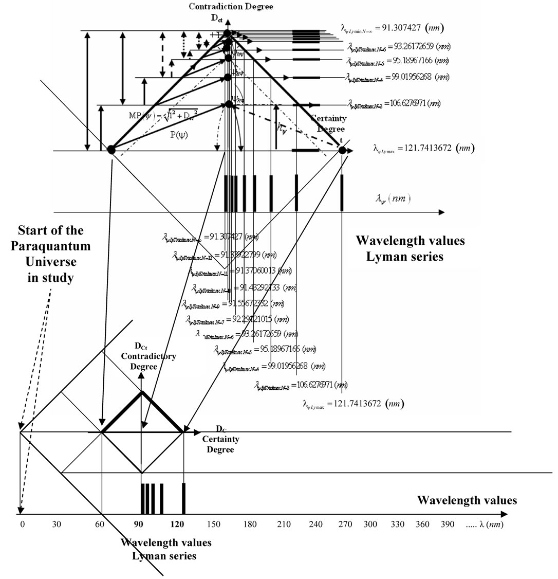
Figure 10. Representation of the Lyman series in a net of lattices of the Paraquantum universe.
the Paraquantum equations can be represented in a Paraquantum universe composed of superposed lattices. A first representation can be made in the series of Lyman, where the wavelength values are exposed in the horizontal axis, according to the Figure 10.
With the values presented in the horizontal axis the Lattice of the Balmer series is superposed to the Lattice of the Lyman series. Figure 11 shows that representation of the Lattices in the net of the Paraquantum universe.
In the same way, the representation of the values of the wavelength of the Paschen series begins in the end of the Balmer series. Figure 12 shows that representation of the
Figure 11. Representation of the Balmer series and Lyman series in the Paraquantum universe.
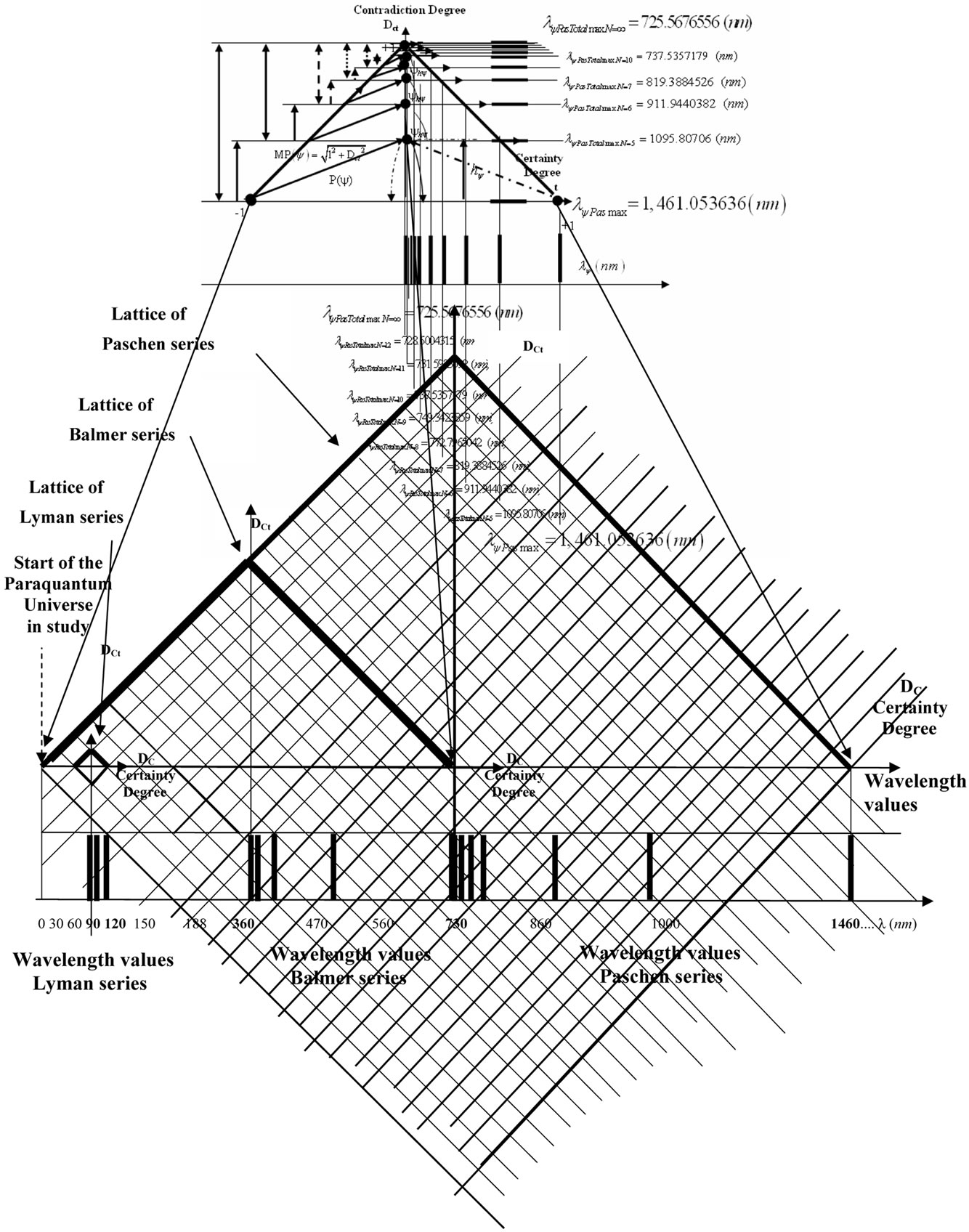
Figure 12. Representation of the Paschen series, Balmer series and Lyman series in the Paraquantum universe.
three Lattices the Paraquantum universe.
Calculations by Paraquantum equations present result where the values of the wavelength of the Brackett series begin in the end of the Paschen series. The same representation happens for the series Pfund and Humphreys.
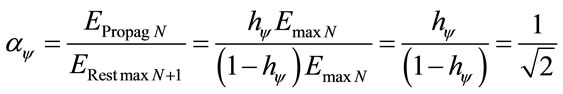
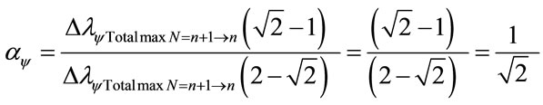
3.6. The Paraquantum Structure Constant αψ
The analysis of the spectrum of radiation of the atom through the Paraquantum Logic shows a constant numeric value obtained by the relationship among the values of the layers of the Lattice. Due to being a constant value that appears in the structure of the Paraquantum Universe it will be denominated of “Paraquantum Structure Constant”, whose symbol will be αψ.
The Paraquantum Structure Constant is calculated in the following way:
Being Equation (24), that result in Energy of Propagation quantized at each layer: 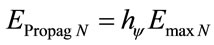
And Equation (30), that result in the remaining energy:

Then:
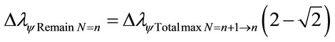
The variation of wavelength value pure for N = n is:
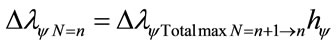
or with :
:

where  is the variation related at Energy of Propagation quantized at each layer.
The variation of wavelength value related at the remaining energy in the Lattice is:
or with :
:
Then, when we consider wavelength values, the Paraquantum Structure Constant is calculated in the following form:
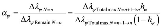
or with :
:
4. Conclusion
In this paper we presented the main concepts of the PQL with applications on analysis of the spectral line emissions of the hydrogen atom. Through the Paraquantum equations we investigated the effects of energy balancing, quantization properties and transiences on the Paraquantum Logical Model in a comparative numerical study which deals with the PQL applied to the Bohr’s Model of the Hydrogen atom. With Paraquantum Equations we made the mathematical relationships of values of energy in the atom of hydrogen and the wavelength calculations in seven series of the radiation spectrum. The values of the wavelengths obtained in the first three series are very close of the values obtained by conventional calculations. The last three series showed values that didn’t approach the results obtained by conventional calculation; however this happened because in this work there were not mathematical rounding in the values and any simplification of the results. In this analysis with the Paraquantum logic was obtained still a numeric value that it relates the layers of the Paraquantum Logical Model. As it presents the action among the structures of the Paraquantum universe it was denominated of Paraquantum Structure Constant, whose symbol is αψ. The results presented in this work open a vast research field to find means of resolution of problems related to physical phenomena using the fundamental concepts of the Paraquantum Logic.
REFERENCES
- S. Jaśkowski, “Propositional Calculus for Contradictory Deductive Systems,” Studia Logica, Vol. 24, No. 1, 1969, pp. 143-157. doi:10.1007/BF02134311
- N. C. A. da Costa, “On the Theory of Inconsistent Formal Systems,” Notre Dame Journal of Formal Logic, Vol. 15, No. 4, 1974, pp. 497-510. doi:10.1305/ndjfl/1093891487
- N. C. A. da Costa and D. Marconi, “An Overview of Paraconsistent logic in the 80’s,” The Journal of NonClassical Logic, Vol. 6, No. 1, 1989, pp. 5-31.
- N. C. A. Da Costa, V. S. Subrahmanian and C. Vago, “The Paraconsistent Logic PT,” Zeitschrift fur Mathematische Logik und Grundlagen der Mathematik, Vol. 37, 1991, pp. 139-148. doi:10.1002/malq.19910370903
- J. I. Da Silva Filho, G. Lambert-Torres and J. M. Abe, “Uncertainty Treatment Using Paraconsistent Logic—Introducing Paraconsistent Artificial Neural Networks,” Vol. 21, IOS Press, Amsterdam, 2010, p. 328.
- J. I. Da Silva Filho, G. Lambert-Torres, L. F. P Ferrara, A. M. C. Mário, M. R. Santos, A. S. Onuki, J. M. Camargo and A. Rocco “Paraconsistent Algorithm Extractor of Contradiction Effects—Paraextrctr”, Journal of Software Engineering and Applications, Vol. 4, No. 11, 2011, pp. 579- 584.
- J. I. Da Silva Filho, A. Rocco, A. S. Onuki, L. F. P Ferrara and J. M. Camargo, “Electric Power Systems Contingencies Analysis by Paraconsistent Logic Application,” International Conference on Intelligent Systems Applications to Power Systems, Niigata, 5-8 November 2007, pp. 1-6,
- C. A. Fuchs and A. Peres, “Quantum Theory Needs No ‘Interpretation’,” Physics Today, Vol. 53, No. 3, 2000, pp. 70-71. doi:10.1063/1.883004
- D. Krause and O. Bueno, “Scientific Theories, Models, and the Semantic Approach,” Principia, Vol. 11 No. 2, 2007, pp. 187-201.
- J. A. Wheeler and H. Z. Wojciech, Eds., “Quantum Theory and Measurement,” Princeton University Press, Princeton, 1983.
- J. I. Da Silva Filho, “Paraconsistent Annotated Logic in analysis of Physical Systems: Introducing the Paraquantum Factor of Quantization hψ,” Journal of Modern Physics, Vol. 2, No. 11, 2011, pp. 1397-1409.
- J. I. Da Silva Filho, “Analysis of Physical Systems with Paraconsistent Annotated Logic: Introducing the Paraquantum Gamma Factor γψ,” Journal of Modern Physics, Vol. 2, No. 12, 2011, pp. 1455-1469.
- P. A. Tipler, “Physics,” Worth Publishers Inc., New York, 1976.
- P. A. Tipler and G. M. Tosca, “Physics for Scientists,” 6th Edition, W. H. Freeman and Company, New York, 2007.
- P. A. Tipler and R. A. Llewellyn, “Modern Physics,” 5th Edition, W. H. Freeman and Company, New York, 2007.