Journal of Modern Physics
Vol. 2 No. 12 (2011) , Article ID: 9040 , 13 pages DOI:10.4236/jmp.2011.212180
Analysis of Physical Systems with Paraconsistent Annotated Logic: Introducing the Paraquantum Gamma Factor γψ
1Santa Cecília University, Group of Applied Paraconsistent Logic, Santos, Brazil
2Institute for Advanced Studies of the University of São Paulo, Térreo, Cidade Universitária, São Paulo, Brazil
E-mail: inacio@unisanta.br
Received August 30, 2011; revised October 9, 2011; accepted October 28, 2011
Keywords: Paraconsistent logic, paraquantum logic, classical physic, relativity theory, quantum mechanics
ABSTRACT
In this paper we use a non-classical logic called ParaQuantum Logic (PQL) which is based on the foundations of the Paraconsistent Annotated logic with annotation of two values (PAL2v). The formalizations of the PQL concepts, which is represented by a lattice with four vertices, leads us to consider Paraquantum logical states ψ which are propagated by means of variations of the evidence Degrees extracted from measurements performed on the Observable Variables of the physical world. In this work we introduce the Paraquantum Gamma Factor γPψ which is an expansion factor on the PQL lattice that act in the physical world and is correlated with the Paraquantum Factor of quantization hψ whose value is associated with a special logical state on the lattice which is identified with the Planck constant h. Our studies show that the behavior of the Paraquantum Gamma Factor γPψ, at the time of reading the evidence Degrees through measurements of the Observable Variables in the physical world, is identical to that one of the Lorentz Factor γ used in the relativity theory. In the final part of this paper we present results about studies of expansion and contraction of the Paraquantum Logical Model which correlate the factors γPψ and γ. By applying these correlation factors, the lattice of the PQL suitable for the universe understudy can be contracted or expanded, allowing the quantization model to cover the several study fields of physics.
1. Introduction
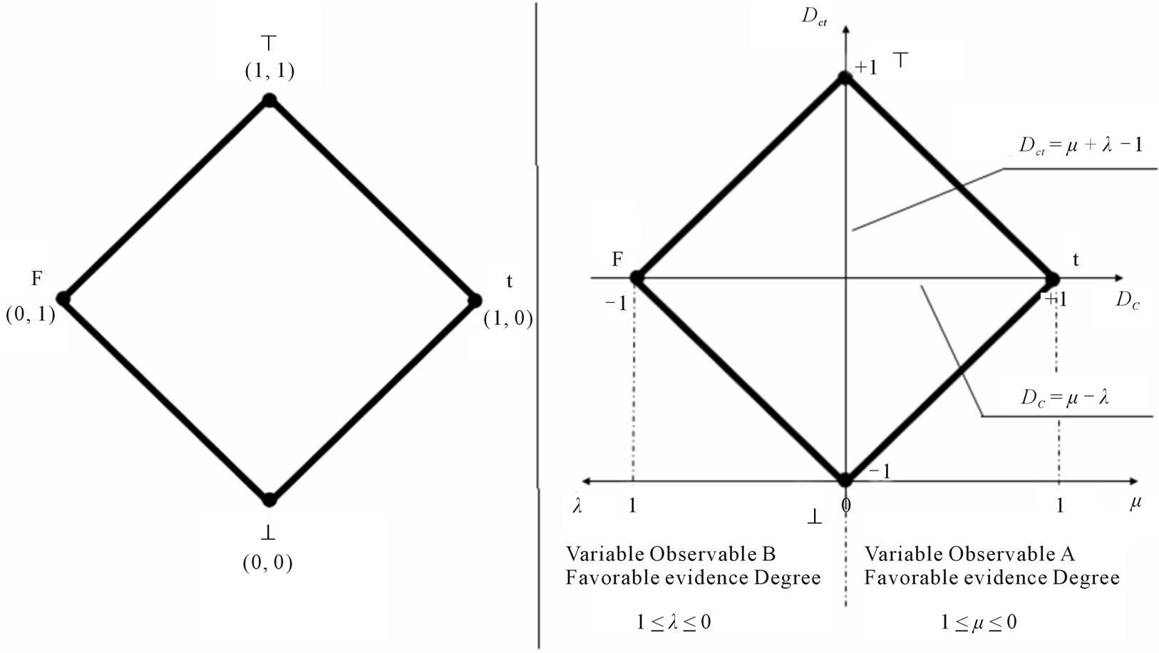
We present in this paper an alternative of modeling physical systems through a non-Classical logic namely the Paraconsistent Logic (PL) whose main feature is the revocation of the principle of non-contradiction [1]. In other words, in its foundation this logic is capable of dealing with contradictory signals [2,3]. Important research has been made in the projects of expert systems based on algorithms based on a non-Classical logic, namely Paraconsistent Annotated logic with annotation of two values (PAL2v) [4]. The applications of PAL2v have been successful in the development of expert systems that have to make decisions based on uncertain or contradictory information [5-7]. In these applications of the PAL2v there was the need of some restrictions on the algorithms because in certain conditions the model presented values which were generated through jumps or unexpected variations [5,7]. Results of more recent research show that the restrictions were imposed on the PAL2v because it has features in its basic structure such that the results obtained can be identified with phenomena watched in the study of quantum mechanics [8]. According to [4] we can obtain through the PAL2v a representation of how the annotations or evidences express the knowledge about a certain proposition P. This is done through a lattice on the real plane with pairs (m, λ) which are the annotations as seen in figure 1(a). With the values of x and y that vary between 0 and 1 and being considered in an Unitary Square on the Cartesian Plane (USCP) [4] we obtain the following final transformation in the lattice of the PAL2v:
 (a) (b)
Figure 1. Lattice of four vertexes and representation Certainty Degree (DC) and Contradiction Degree (Dct).
 (1)
(1)
According to the language of the PAL2v we have:
x = m is the Favorable evidence Degree.
y = λ is the Unfavorable evidence Degree.
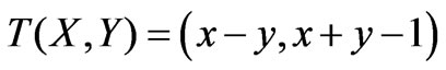
As seen in figure 1(b) the first coordinate of the transformation (1) is called Certainty Degree DC.
 (2)
(2)
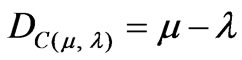
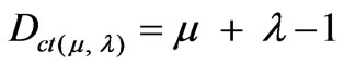
The second coordinate of the transformation (1) is called Contradiction Degree Dct.
 (3)
(3)
The second coordinate is a real number in the closed interval [−1,+1].
The y-axis is called “axis of the contradiction degrees”.
Since the linear transformation T(X,Y) shown in (1) is expressed with evidence degrees μ and λ, from (2), (3) and (1) we can represent a Paraconsistent logical state eτ into Lattice τ of the PAL2v, such that:
 (4)
(4)
or
 (5)
(5)
where: eτ is the Paraconsistent logical state.
DC is the Certainty Degree obtained from the evidence degrees μ and λ.
Dct is the Contradiction Degree obtained from the evidence degrees μ and λ.
2. The Paraquantum Logic—PQL
Based on the previous considerations about the PAL2v [4,9-10], we present the foundations of the Paraquantum Logics PQL as follows.
2.1. The Paraquantum Function ψ(PQ) and the Paraquantum Logical State ψ
A paraquantum logical state ψ is created on the lattice of the PQL as the tuple formed by the certainty degree DC and the contradiction degree Dct. Both values depend on the measurements perfomed on the Observable Variables in the physical environment which are represented by μ and λ. Equations (2) and (3) can be expressed in terms of μ and λ as follows:
 (6)
(6)
 (7)
(7)
A Paraquantum function y(Py) is defined as the Paraquantum logical state y:
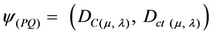 (8)
(8)
For each measurement performed in the physical world of μ and λ, we obtain a unique duple 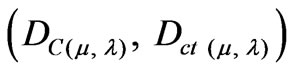 which represents a unique Paraquantum logical state ψ which is a point of the lattice of the PQL, where on the vertical axis of contradiction degrees:
 is the contradictory extreme Paraquantum logical state of Inconsistency T.
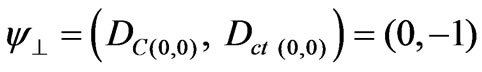 is the contradictory extreme Paraquantum logical state of Undetermination ^.
On the horizontal axis of certainty degrees, the two extreme real Paraquantum logical states are:
 is the real extreme Paraquantum logical state which represents Veracity t.
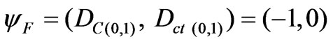 is the real extreme Paraquantum logical state which represents Falsity F.
2.3. The Vector of State P(ψ)
A Vector of State P(ψ) will have origin in one of the two vertexes that compose the horizontal axis of the certainty degrees and its extremity will be in the point formed for the pair indicated by the Paraquantum function  .
.
If the Certainty Degree is negative (DC < 0), then the Vector of State P(ψ) will be on the lattice vertex which is the extreme Paraquantum logical state False: ψF = (−1,0).
If the Certainty Degree is positive (DC > 0), then the Vector of State P(ψ) will be on the lattice vertex which is the extreme Paraquantum logical state True: ψt = (1,0).
If the certainty degree is nil (DC = 0), then there is an undefined Paraquantum logical state ψI = (0.5;0.5).
Figure 2 shows a point (DC, Dct) where DC = f(μ, λ) and Dct = f (μ, λ) which represents a Paraquantum logical state ψ on the lattice of states of the PQL.
Given a current Paraquantum logical state ψcur defined by the duple (DC, Dct), the Vector of State P(ψ) is computed by:
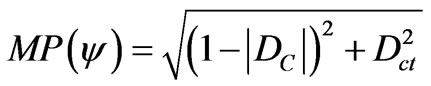
1) For DC > 0 the real Certainty Degree is computed by: .
.
Therefore:
 (9)
(9)
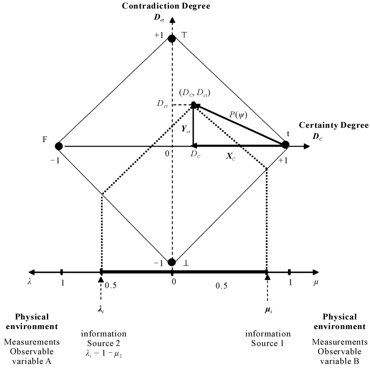
Figure 2. Vector of State P(ψ) representing a Paraquantum logical state ψ on the Paraquantum lattice of states on the point (DC, Dct).
where:
DCψR = real Certainty Degree.
DC = Certainty Degree computed by (6).
Dct = Contradiction Degree computed by (7).
2) For DC < 0, the real Certainty Degree is computed by: 
Therefore:
 (10)
(10)
where:
DCψR = real Certainty Degree.
DC = Certainty Degree computed by (6).
Dct = Contradiction Degree computed by (7).
3) For DC = 0, then the real Certainty Degree is nil:
 .
.
The intensity of the real Paraquantum logical state is computed by:
 (11)
(11)
The inclination angle ay of the Vector of State which is the angle formed by the Vector of State P(y) and the x-axis of the certainty degrees is computed by:
 (12)
(12)
The degree of intensity of the contradictory Paraquantum logical state ψctrψ is computed by:
 (13)
(13)
where: μctrψ = intensity degree of the contradictory Paraquantum logical state.
Dct = Contradiction Degree computed by (7).
Since the Paraquantum analysis deals with Favorable and Unfavorable evidence Degrees m and l of the measurements performed on the physical world, these variations affect the behavior and propagation of the superposed Paraquantum logical states ysup on the lattice of the PQL.
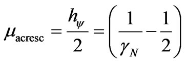
The Paraquantum logical state of quantization yhy which is located in the equilibrium points of the lattice can be obtained through trigonometric analysis.
2.4. The Paraquantum Factor of quantization hy
When the superposed Paraquantum logical state ysup propagates on the lattice of the PQL a value of quantization for each equilibrium point is established. This point is the value of the contradiction degree of the Paraquantum logical state of quantization yhy such that:
 (14)
(14)
where:
hy is the Paraquantum Factor of quantization.
The factor hy quantifies the levels of energy through the equilibrium points where the Paraquantum logical state of quantization yhy, defined by the limits of propagation throughout the uncertainty of the PQL, is located. Figure 3 shows the interconnections between the factors and its characteristics, in which they delimit the Region of Uncertainty in the Lattice of PQL.
In a process of propagation of Paraquantum logical state y, it happens that in the instant that the superposed Paraquantum logical state ysup reaches the representative points of the limiting factors of the uncertainty region of the PQL, the Certainty Degree (DC) remains zero but the real Certainty Degree (DCyR) will be increased or decreased from zero and this difference corresponds to the effect of the Paraquantum Leap. At the instant that the superposed Paraquantum logical states ysup visit the Paraquantum logical state of quantization yhy, the real Certainty Degree will have variations of the form:
 (15)
(15)
We observed that when the Paraquantum logical states ysup visit the Paraquantum state of quantization yhy established by the Paraquantum Factor of quantization hy, the Paraquantum Leap happens. In the study of the PQL, when the propagation happens only in this point, the lattice is called fundamental lattice of transition frequency level N = 1.
Since that for the fundamental lattice of the PQL, the number of times of application of the Paraquantum Factor of quantization hy is N = 1, then, for a contraction or expansion, the number of times will be greater than 1. Generalizing, we have that the Paraquantum Factor of quantization hy expands or contracts the lattice of the PQL N times such that:
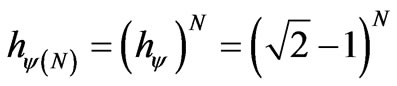 (16)
(16)
where:
N is an integer greater than 1.
The Paraquantum Factor of quantization hψ can be used to correlate the values of quantities between the physical environment and the Paraquantum universe represented by the lattice of the PQL. The successive applications of hψ leads to a formula of expansion of the initial lattice which, keeping its referential on the horizontal axis can be expressed for level N as follows:
 (17)
(17)
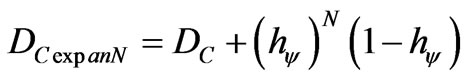 (18)
(18)
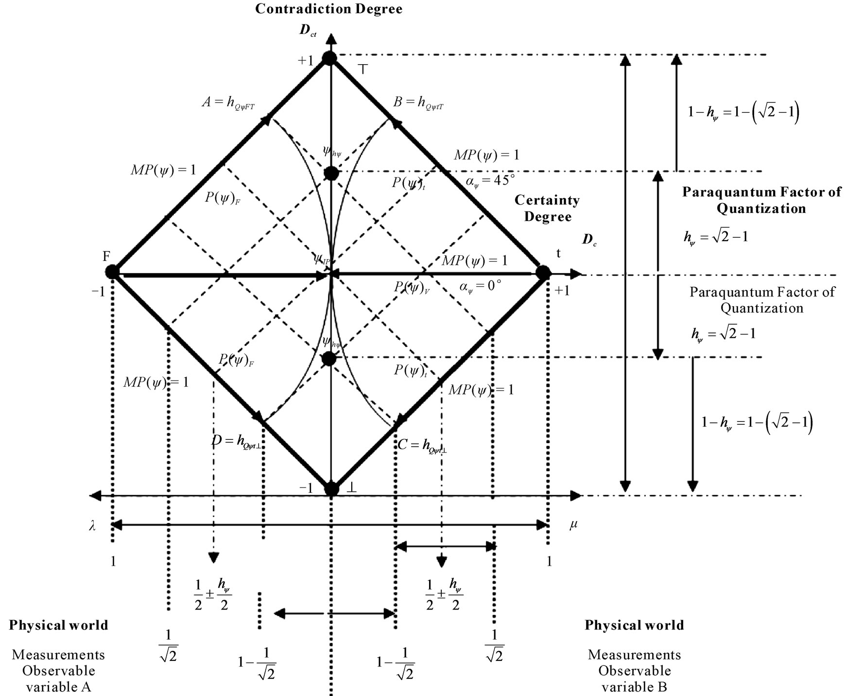
Figure 3. The paraquantum factor of quantization hy related to the degrees of evidence obtained in the measurements of the observable variables in the physical world.
Figure 4 shows the expansion of the fundamental lattice of the PQL with expansion order . The largest expansion will feel with N = 1 and the expansions in reference to the initial Lattice will be smaller as N increases. It is verified that the increase due to expansion is symmetrical, therefore the value that expands for the vertex T of Inconsistency logical state with, hψT →
 →···
→··· it is equal value to the that expands for the vertex of the Undetermination ^ logical state with, hψ^ →
 →···
→··· .
.
In that way, the contraction equation can be presented for a level N, such that:
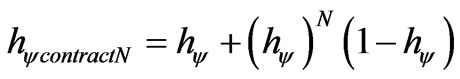 (19)
(19)
 (20)
(20)
with N ³ 1 positive and belonging to the integer number set.
where: DCcontractN = contracted Certainty Degree.
DC = Certainty Degree computed by (9).
hy = the Paraquantum Factor of quantization.
N = level of contraction frequency, or number of times of application of hψ.
In the figure the Paraquantum logical states indicates that the Uncertainty Region of PQL is dependent of the level of transition frequency N that acts in the Paraquantum Factor of quantization hψ, such that:
 (21)
(21)
N = integer positive ≥ 1 where: ΔψIP is the variation around the Paraquantum logical state of Indefinition pure.
N is the level of contraction frequency, or number of times of application of hψ.
In relation to the physical world, the contraction of the
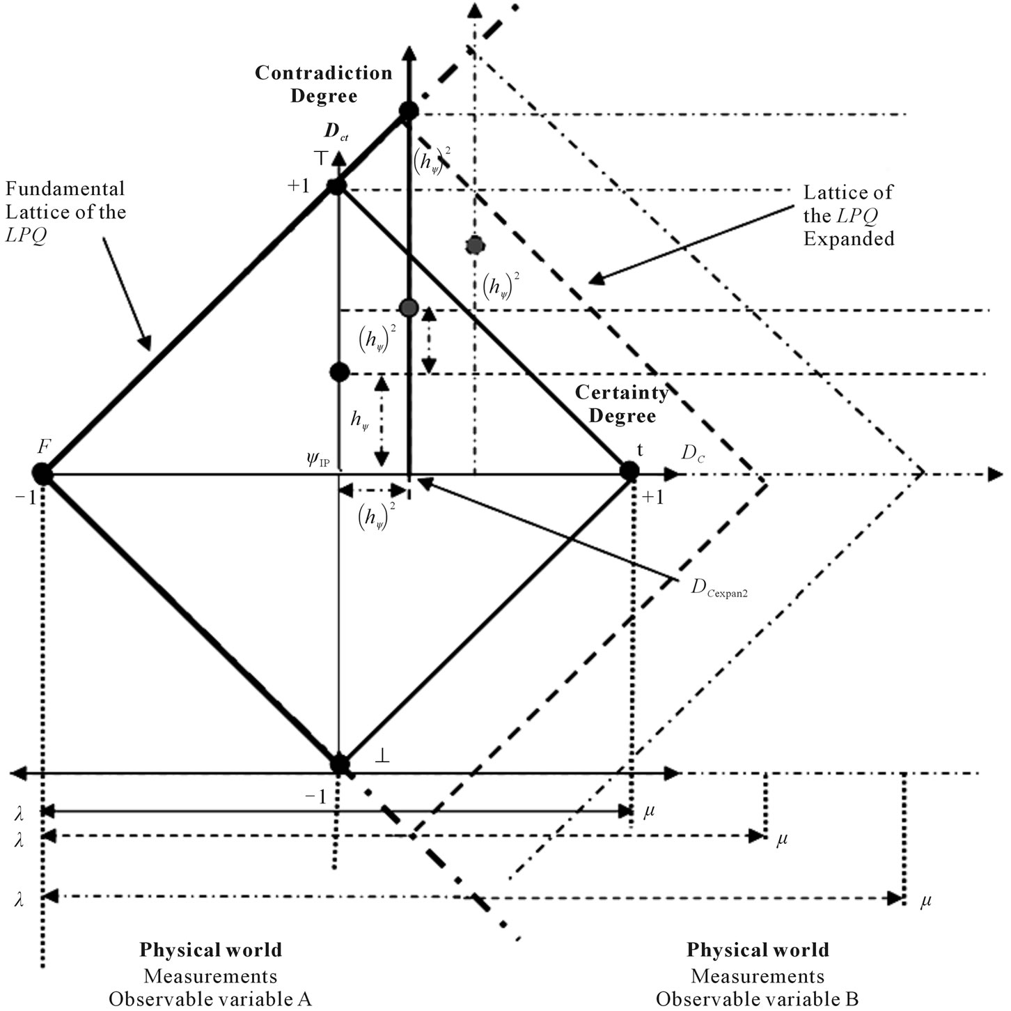
Figure 4. Expansion of the fundamental lattice of the PQL with expansion order .
.
Fundamental lattice, that it happens starting from the Paraquantum logical state of Indefinition pure ψIP, have their values obtained through:
Favorable evidence Degree:  and Unfavorable evidence Degree:
where N is integer positive ≥1, what indicates the level of frequency of transition of the PQL lattice.
3. Paraquantum Analysis in Physical Systems
Based on the above equations we present the Paraquantum Logic (PQL) as a logical solution for resolution of phenomena modeled by the laws of Physics [2,4,9,11]. In order to develop this study, we start its application base on assumptions made from experimental observations of the Newton laws [12-15]. Doing this the PQL will allow, through the Paraquantum Logical Model, the mathematical applications to be extended to all fields of the physical science.
3.1. The Newton’s Second Law
The idea of the second Newton law is that when a resultant of forces acts on a body, this body will receive an acceleration which is proportional to Force (F) and inversely proportional to its mass (m) [13,15]. When the law is expressed as a mathematical equation, this statement depends on a value that adjusts or defines this proportionality between the largenesses such that:
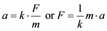 (22)
(22)
where:
a is the acceleration or the ratio through which the velocity of the body changes along time.
F is the resultant of all forces acting on the body.
m is the mass of the body.
k is a factor of adjustment of proportionality.
When mathematically considered the second Newton law expressed the relation between the largenesses force, mass and acceleration. It is well known that the adjusts of measure units with respect to the Newton laws were performed in a way that the proportionality constant k, from the second law and represented in (22), became 1 in the International System of Units (SI) largely used nowadays [8,16]. The International System of Units (SI) uses three fundamental largenesses of the Metric Systems: mass, length and time.
3.2. Correlation between the Units of the British and the International Systems
In order to apply the Paraquantum Logics PQL on physical systems it is important to study Newton’s laws that relate the involved physical largenesses (force, mass and acceleration) with the British System of units as well as the implications with respect to their transformations to the International System of Units (SI) [16]. In the British System of units those largenesses considered fundamental are defined as: force, length and time. Because of that there is no freedom to choose units for force and acceleration that must be used, however, to define the unit for mass so large or so small as desired. Doing so, the value of the proportionality constant k in (22), which represents the second Newton law, depends on the value of the unit chosen for mass.
For the unit of force when the proportionality factor k acts on the mass, where the force and the acceleration are 1 in the International System of units (SI), the equation that expresses the poundal of the British System of units [16,17]is expressed by:
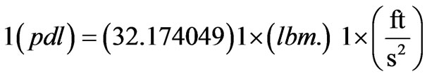 (23)
(23)
Comparing (22) which represents Newton’s second law with (23) which represents (22) expressed in the form of Newton’s second law in units of the British System, we have the inverse value of the proportionality constant k:
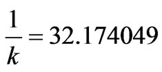 .
.
The slug is compatible with the British System of units where the unit of force (and weight) is the pound. If 1 slug is 14.5939 kg, then the corresponding to 1/32.174049 of the slug in the British System of units such as force will be obtained in the International System of units (SI) by the following equality:

We repeat the above again but now using the corresponding values from the International System of units (SI) where the unit for force is the Newton (N). In this case, (23) can be expressed by:
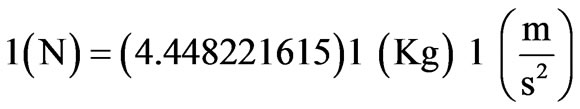 (24)
(24)
We obtain from (22), which represents the second Newton law, comparing with (24), which represents second Newton law in the International System of units (SI), the inverse value of the proportionality factor k such that: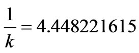 .
.
Equating (23) and (24), force and acceleration become 1. In this case:
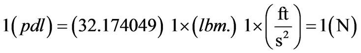

We observe in the equality that for the International System of units (SI) to present the value of force F in an unit of Newton, an adjustment of the value of mass of the International System of units (SI) was needed. An adjustment was also necessary in the British System of units when the transformation from feet to meters was done. So, in order to obtain 1N (Newton) of force, with mass and acceleration 1 in the British System we write:

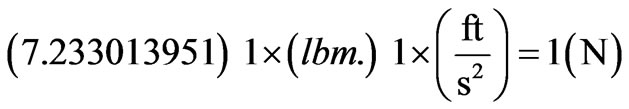
Comparing with (22), which represents the second Newton law, the factor of proportionality adjustment is:
 which is a factor of proportionality adjustment of the British System of units:
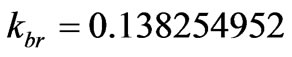
In the same way in order to obtain 1 poundal (pdl) of force, with mass and acceleration 1 in the International System of units (SI) we write:
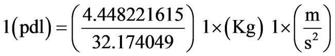
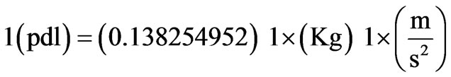
Comparing with (22), which represents the second Newton law, we have that:

which gives us a factor of proportionality adjustment in the International System of units: 
Comparisons and analogies between the Systems of units lead us to relations and values that made the proportionality factor k of (22), which represents the second Newton law, to be 1 in the International System of units (SI). The analysis of physical systems through the Paraquantum Logics PQL is started with the receiving of information from the physical environment through the Evidence Degrees µ and λ obtained from measurements of observable variables [18]. The values of the Evidence Degrees extracted from the information sources are normalized [4][19], therefore, they are in the closed real interval between 0 and 1. In order to build a Paraquantum Logical Model it is necessary to impose these normalization conditions to the values of the factors of proportionality adjustment kIS that appear in the equations related to the second Newton law as seen in (22). The adjustments needs the factor of proportionality adjustment kbr of the British System of units to be multiplied by 10 and the factor of proportionality kSI of the International System of units (IS) to be divided by 10. Therefore:
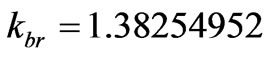 and
and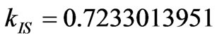 .
.
The fundamental theory of the PQL formalizes the Paraquantum logical states ψ which propagate through the fundamental Lattice always in diagonal form, building internal propagation lattices. Doing so, the values of the factors of proportionality adjustment k obtained from the experimental physics related to the Newton second law, which were treated in this paper, are very close to the ones expected in the theory and formalization of the PQL.
This allows the characterization of identifying properties among the natural processes of results obtained from experiments with the theory that is foundational to the PQL.
The theoretical and experimental values show that the PQL is a logic capable of creating models that can represent the physical phenomena with a good approximation of the values obtained through the equations representing the second law of Newton. So, it is possible to adapt the factors of proportionality adjustment k obtained for the Paraquantum Logical Model as follows:
 and
and 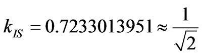
Considering that the values of k were obtained from arbitrary measurements, whose values were adapted along the years with practical applications, the differences are low.
3.3. Newton Gamma Factor
We consider that applying the PQL in the analysis of physical quantities will produce through its Paraquantum Logical Model results identified with the International System of Units (SI). The proportionality factor which will affect the analysis when we want to express values in the British System will be: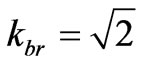 .
.
Considering that the values read from the observable variables, which are related to the evidence degrees of the fundamental quantities of physics, are obtained from measurement devices which are graduated in units from the International System of Units (SI), we have to multiply the obtained values by .
.
These considerations show that the application of the PQL for the analysis of physical systems provides us with a Paraquantum logical model which produces quantization of  on the fundamental quantities of physics, when these are used as Observable Variables in the physical world, from where the evidence degrees are extracted. We observe that the quantization of
  on the evidence Degrees µ and λ produces a quantization of
  on the axis of contradiction degrees on the lattice of the PQL.
This corresponds to the Paraquantum Factor of quantization  obtained on the equilibrium point where the Paraquantum logical state of quantization
  is located. In the application of the Paraquantum Logical Model in broad areas of physics, the factor
  as well as its inverse will be largely used to perform adjustments needed to the natural proportionality that exists between physical quantities and adjustment of unitary values between unit systems. Due to its importance, well call this value Newton Gamma Factor and represent it by
 . Therefore, for the classical logic applied in the Paraquantum Logical Model, we have Newton Gamma Factor
 .
.
3.4. Newton Gamma Factor γN and Lorentz Factor γ
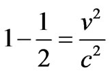
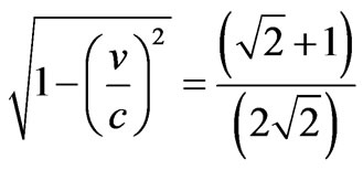
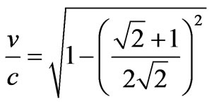
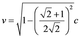
When we compare the Lorentz factor  applied in the Relativity Theory to the Newton Gamma Factor
 , the latter is considered to be well-behaved because it does not change with the variations of velocity related to the light speed c in the vacuum. If we consider the equality
 , we have:

v is the velocity of the body in relation to the light speed c in the vacuum.
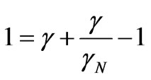
The equality can be rewritten removing the square root of both sides and isolating 1:

Manipulating the equation we have:
 or
or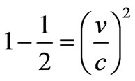 .
.
The velocity of the body is expressed as a fraction of the light speed c in the vacuum so:
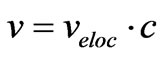
where:  is the value of constant velocity of the body in comparison with the light speed in the vacuum such that
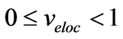 .
.
According the Relativity Theory,  is expressed as a constant smaller or equal the light speed in the vacuum. We observe that the equation relating Newton and Lorentz factors can be written as follows:
or 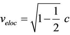 resulting:
  which is identified in the interval as being a constant value smaller or equal the light speed c in the vacuum. Therefore, this is the quantitative value of the velocity v of the body in relation to the light speed c in the vacuum for which the Newton and Lorentz factors coincide.
4. The Paraquantum Gamma Factor γPψ
The equality condition between Newton Gamma Factor  from classical mechanics and the Lorentz factor
  from the Relativity Theory which resulted in the equation
 . This shows that that equality expresses a strong bond between values of fundamental quantities of two important areas of physics. Classical physics and Relativity Theory can be represented jointly in the Paraquantum logical model through only one factor. This factor which links Newton’s theories to the restricted relativity theory is called Paraquantum Gamma Factor
  which we study in the following.
4.1. Application of Newton Gamma Factor
Equation (21) expresses the variation of the value of the Favorable evidence Degree µ extracted from measurements performed on Observable Variables in the physical environment, correlating to the Paraquantum Factor of quantization hψ on the lattice of the PQL. Equation (21)
is as follows: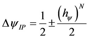 .
.
Since , this equation can be written just considering the extraction of the Favorable evidence Degree such that:
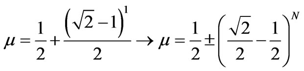
or 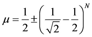
If we express it using the Newton Gamma Factor, we have: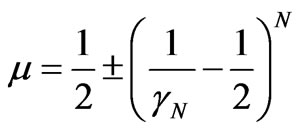 .
.
We can express the increased value of each quantization in an expansion as being:
 (25)
(25)
The expression (21) of the value of variation of the Favorable evidence Degree µ extracted from measurements performed on Observable Variables in the physical world, correlating the Paraquantum Factor of quantization hψ on the lattice of the PQL, shows that  for a situation before the application N = 1, this is, before the condition was analyzed.
The equation that results this value informs the present condition that there was an evidence degree µ such that when multiplied by the previous value, the result 
was obtained. This condition previous to analysis this value can be mathematically expressed through multiplications of inverse values of the Newton Gamma Factor.
An initial application before the fundamental lattice resulted the previous value .
.
We have that the previous condition was produced by:
 →
→ →
→
We consider that in the expansion of the lattice, there will always be an increase proportional to  to the value of each analyzed situation.
This means that, in an expansion process, at each quantization there will be an increase to the present value of the evidence degree corresponding to the inverse value of the Newton Gamma Factor. So, in the previous equation we can obtain results where the application of the inverse value of Newton Gamma Factor is restricted only to the increased value of the fundamental lattice such that:

In a process of expansion where we consider quantizations in successive applications of inverted values of the Newton Gamma Factor and where the evidence degree in the beginning represents Indefinition, we can do the following: for the first application of the inverted value of the Newton Gamma Factor we can write its present value with increase with condition N = 1 such that:
 which represented by the Newton Gamma Factor is:
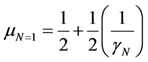 .
.
According to the same procedure of expansion of the lattice, keeping the inverted value of the Newton Gamma Factor in the successive applications, we obtain:
For N = 2
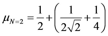
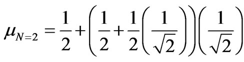 →
→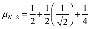 →
→
which represented by the Newton Gamma Factor is:
For N = 3
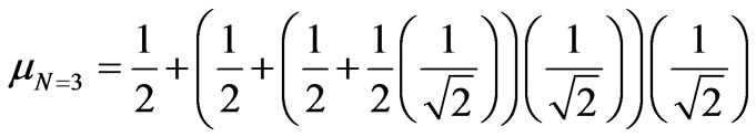

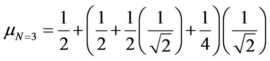 →
→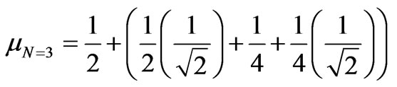 →
→
which repre-sented by the Newton Gamma Factor is:
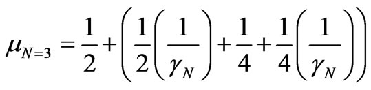 .
.
For N = 4
 →
→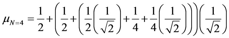 →
→
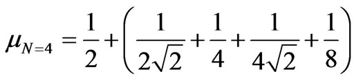 →
→ →
→
which represented by the Newton Gamma Factor is:
 .
.
For N = 5
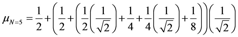 →
→ →
→
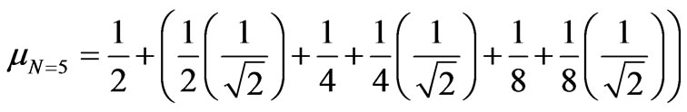 →
→
which represented by the Newton Gamma Factor is:
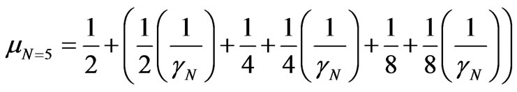 .
.
For N = 6
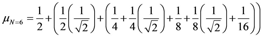 →
→
which represented by the Newton Gamma Factor is:
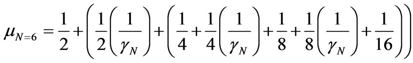 .
.
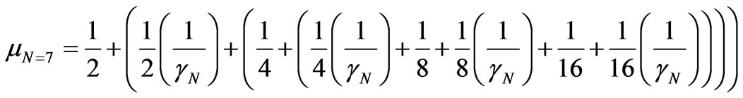
For N = 7
 →
→
which represented by the Newton Gamma Factor is:
For N = 8
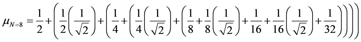
which represented by the Newton Gamma Factor is:

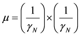
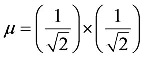
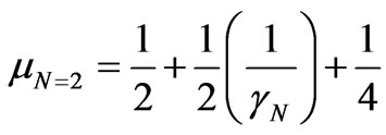
We observe that the process of application of the inverted value of the Newton Gamma Factor is the following geometric progression:

with values: 
and
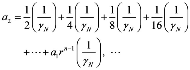
We observe that the following sum:
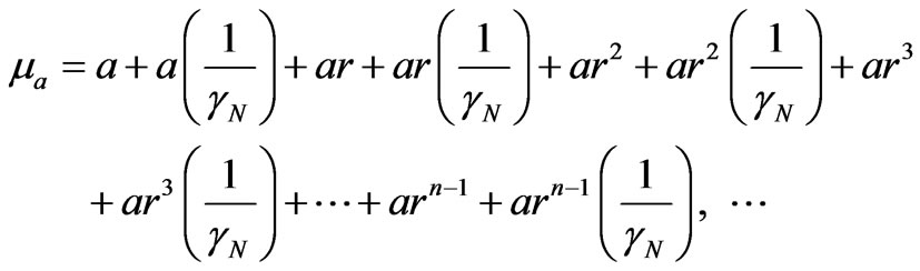
is the infinite series. If we substract 1 from it, it will become the binomial expansion of the Lorentz Factor  used in the Relativity Theory such that:
 ↔
↔ 
We can identify the Lorentz Factor  in the infinite series of the binomial expansion correlated to the series obtained from successive applications of the Newton Gamma Factor
  such that:
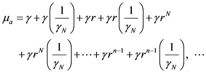
only for odd integer numbers.
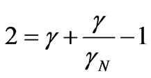
We identify a correlation value of the Paraquantum logics which we call Paraquantum Gamma Factor  such that:
 (26)
(26)
where:
 is the Newton Gamma Factor such that:
 is the Lorentz Factor, such that :
 .
.
If the speed v of the body is correlated to the light speed c in the vacuum, which is the maximum value of velocity in the Relativity Theory [8][20-22] and a limit to the construction of a lattice of the PQL, then the Paraquantum Gamma Factor  is applied to the computation of the evidence degrees extracted from the Observable Variables in the physical environment.
4.2. Variations of the Paraquantum Gamma Factor
As it was done for the Newton Gamma Factor, the value of the Paraquantum Gamma Factor  is applied from the condition of Indefinition in the Paraquantum analysis, where the analyzed situation is identified by the Favorable evidence Degree
  and by the Unfavorable evidence Degree
 .
.
We observe that with the analysis of (26) the Paraquantum Gamma Factor  depends only on the value contained in the Lorentz Factor
  and therefore on the velocity v of the body in relation to the speed light c in the vacuum. When we use the Paraquantum Gamma Factor
 , the velocity v of the body is always correlated to the speed light c in the vacuum, so its value depends on the Lorentz Factor
  which, according to the Relativity Theory, changes with the increase or decrease of the velocity v [8,15].
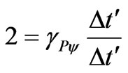
The equation (26) for a quantitative paraquantum analysis of the time and velocity can be compared to the Time dilation equation of the special relativity theory [8,15].
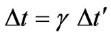 (27)
(27)
where:  is the variation value of the time measured in the referential point.
 is the variation value of the time measured in the body point in movement when is measured in the referential point.
 = Lorentz Factor, such that:
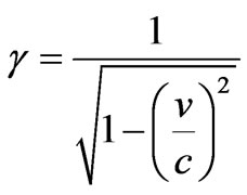
4.3. Selected Examples of Application of the Paraquantum Gamma Factor
Some selected examples that deal with the application of the Paraquantum Gamma Factor in equation (26) and involving the time dilation equation (27) of the theory of relativity are presented to follow.
Example of Application
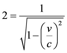
Calculate the value of the velocity that a body must be in relation to the speed of the light in the vacuum, in the following conditions:
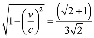
1) So that the time observed in the referential point is the double when calculated by the Time dilation equation of the special relativity theory.
Resolution:
 so that
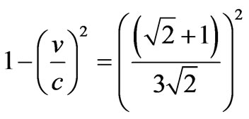
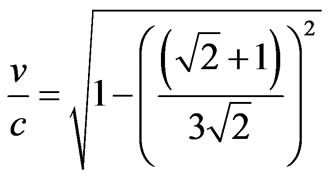
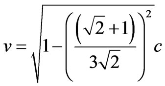
From the equation (27) of the special relativity theory, then: 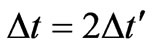
 →
→ →
→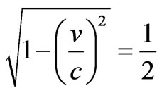 →
→ →
→ →
→
the value of the velocity is:

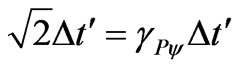
Applying the Paraquantum Logical Model by equation (26): 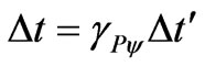 then:
then:
 →
→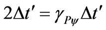 →
→ →
→
Therefore the measured time will be the double when the Paraquantum Gamma Factor will be equal the 2.
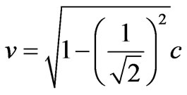
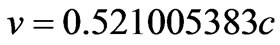
As: 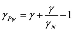 then:
then:
 →
→ →
→ →
→ →
→
the value of the velocity is: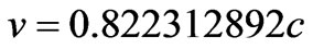 .
.
2) So that the time observed in the referential point is  larger when calculated by the Time dilation equation of the special relativity theory.
Resolution:
 so that
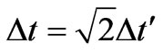
From the equation (27) of the special relativity theory, then:
 →
→ →
→
the value of the velocity is: .
.
Applying the Paraquantum Logical Model by equation (26):

Then:  →
→ →
→ .
.
Therefore, the measured time will be  when the Paraquantum Gamma Factor will be equal
 .
.
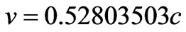
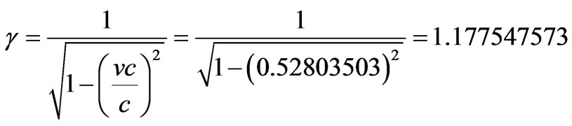
As:  then:
then:
 →
→ →
→
 →
→
the value of the velocity is: 
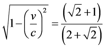
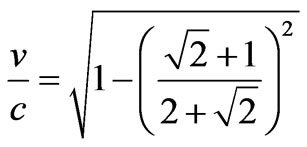
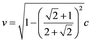
3) So that the time observed in the referential point is equal when calculated by the Time dilation equation of the special relativity theory.
Resolution:
 so that
From the Equation (27) of the special relativity theory, then:
 →
→ →
→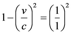 →
→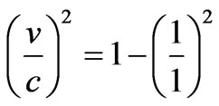 →
→
the value of the velocity is: .
.
Applying the Paraquantum Logical Model by equation (26):

Then:  →
→ →
→ .
.
Therefore the measured time will be equal when the Paraquantum Gamma Factor will be equal 1.
As: then:
then:
 →
→
 →
→
the value of the velocity is:
 .
.
4.4. Limits of the Paraquantum Gamma Factor and Dependence of the Lorentz Factor
Select examples show that the independence condition to get a unitary Lorentz Factor happens only when the velocity v is too low in compared to the light speed c in the vacuum.
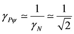
The limits of the Paraquantum Gamma Factor and its dependence with the variation of the Lorentz Factor are presented. It was verified in example c) that the unitary Paraquantum Gamma Factor ( ) happens when the speed value v of the body, in relation at the speed c of the light in the vacuum, to reach the value of:
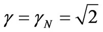
In this condition of the value speed of the body the value of the Lorentz Factor is calculated:
 .
.
Through the equation (26) the value of the Paraquantum Gamma Factor is: 

that results in its unitary value: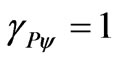 .
.
From this condition if the speed value of the body to diminish, then the Paraquantum Gamma Factor will be minor who the unit until reaching the boundary-value, which is the inverse value of the Factor Gamma of Newton. However, the Lorentz Factor is who limits the Paraquantum Gamma Factor . This condition becomes the Paraquantum Gamma Factor
  a relativistic factor.
4.5. Discussion
We observe that with this condition the result is a value of Paraquantum Gamma Factor  very close to the inverted value of the Newton Gamma Factor
  such that, when:
 →
→
The inverted value of the Paraquantum Gamma Factor  in the Newtonian universe has practically the same effect as the Newton Gamma Factor
 . On the other hand, a careful analysis of the phenomenon shows that the effect of the Paraquantum Gamma Factor
  is initiated from the instant we consider an object with velocity v related to the light speed c in the vacuum.
When the Lorentz Factor  increases in such way that its value becomes the Newton Gamma Factor
 , then the value of the Paraquantum Gamma Factor
  will be the value of the Newton Gamma Factor
 . Under these conditions, the velocity v of the body compared to the light speed c in the vacuum will be the inverted value of the Newton Gamma Factor
 . Therefore, for:
 →
→ and
and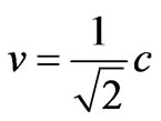 .
.
When the velocity v of the body compared to the light speed c in the vacuum has a value greater than the inverted value of the Newton Gamma Factor , then the value of the Lorentz Factor
  and also the value of the Paraquantum Gamma Factor
  are above
 .
.
Under these conditions the Lorentz Factor  and the Paraquantum Gamma Factor
  will have values varying in a way which is approximate to the results obtained by the Relativity Theory and computations done with (27).
In the Newtonian world the choice of using the Paraquantum Gamma Factor  or the inverted value of the Newton Gamma Factor
  is irrelevant because they are very close values. However, we observe that as the velocity v f the body (considered in relation to the light speed c in the vacuum) increases, there is a significant increase of the Paraquantum Gamma Factor
 . After a certain value of v, the Paraquantum Gamma Factor
  becomes important in the computation of quantities, while the inverse value of the Newton Gamma Facto
  remains the same. The use of the Paraquantum Gamma Factor
  allows computations, which correlate values of the Observable Variables to the values related to quantization through the Paraquantum Factor of quantization hψ, to be performed in any area of study of physical science. Therefore the applications of
  go from the Theory of Relativity to the studies of Quantum Mechanics. This means that variations in the values of the evidence degrees are due to relativistic-type phenomena which are expressed by the Paraquantum Gamma Factor
 . So, the Paraquantum Gamma Factor
  will have influence on the computation of states and on the intensity of measures of physical quantities analyzed in the Paraquantum world represented in the lattice such as velocity, acceleration, energy and power.
5. Conclusions
Based on the concepts of the Paraquantum logics PQL we did in this work a detailed study about the existing correlations between the physical world represented by the values of the evidence degrees and the Paraquantum world, represented by the lattice of the PQL. The equations and forms of dealing with representative values of physical systems considered on the lattice of the PQL allowed to obtain behavioral characteristics of Paraquantum logical states ψ which produce quantitative results affected by the measurements performed on the Observable Variables in the physical environment.
The results of the action of these factors which originated in the application methodology of the PQL in the analysis of physical systems show that the behavior of the Paraquantum Gamma Factor , at the extraction of evidence Degrees through measurements on the Observable Variables of the physical world, is identical to the behavior of the Lorentz Factor
  used in the Relativity Theory.
The correlation between the Paraquantum Gamma Factor , which acts on the measurements performed at the extraction of evidence degrees in the physical world, with the Paraquantum Factor of quantization hψ, allows that the Paraquantum logical model to be capable of analyzing physical quantities in a quantitative fashion.
The model standardizes analysis and interpretations and allows that these applications to be extended to all study areas of physics which are considered incompatible because of existing contradictions in computations. The direct applications in the solution of problems applying the Paraquantum Logical Model in the Newtonian physics and in the physics that covers the theories of quantum mechanics and relativity will be presented in future papers.
6. Acknowledgements
The author thanks INESC—Institute of Engineering of Systems and Computers of Porto, Portugal, in particular researcher Prof. Jorge Correia Pereira for the support during this research.
REFERENCES
- N. C. A. Da Costa and D. Marconi, “An Overview of Paraconsistent Logic in the 80’s,” The Journal of Non-Classical Logic, Vol. 6, No. 1, 1989, pp. 5-32.
- D. Krause and O, Bueno, “Scientific Theories, Models, and the Semantic Approach,” Principia, NEL—Epistemology and Logic Research Group, Federal University of Santa Catarina (UFSC), Santa Catarina, 2007, pp. 187- 201.
- N. C. A. Da Costa, V. S. Subrahmanian and C. Vago, “The Paraconsistent Logic PJ,” Mathematical Logic Quarterly, Vol. 37, No. 9-12, 1991, pp. 139-148. doi:10.1002/malq.19910370903
- J. I. Da Silva Fiho, G. Lambert-Torres and J. M. Abe, “Uncertainty Treatment Using Paraconsistent Logic: Introducing Paraconsistent Artificial Neural Networks,” IOS Press, Amsterdam, 2010, p. 328.
- J. I. Da Silva Filho, A. Rocco, A. S. Onuki, L. F. P. Ferrara and J. M. Camargo, “Electric Power Systems Contingencies Analysis by Paraconsistent Logic Application,” International Conference on Intelligent Systems Applications to Power Systems, Toki Messe, 5-8 November 2007, pp. 1-6. doi:10.1109/ISAP.2007.4441603
- J. I. Da Silva Filho, A. Rocco, M. C. Mario and L. F. P. Ferrara, “PES-Paraconsistent Expert System: A Computational Program for Support in Re-Establishment of the Electric Transmission Systems,” Proceedings of VI Congress of Logic Applied to Technology, Santos, 21-23 November 2007, p. 217.
- J. I. Da Silva Filho, A. Rocco, M. C. Mario and L. F. P. Ferrara, “Annotated Paraconsistent Logic Applied to an Expert System Dedicated for Supporting in an Electric Power Transmission Systems Re-Establishment,” 2006 IEEE PES on Power Systems Conference and Exposition, Atlanta, October 29 2006-November 1 2006, pp. 2212- 2220.
- P. A. Tipler and A. Llewellyn, “Modern Physics,” 5th Edition, W. H. Freeman and Company, New York, 2007.
- J. M. Abe and J. I. Da Silva Filho, “Inconsistency and Electronic Circuits,” In: E. Alpaydin, Ed., Proceedings of EIS’98 International ICSC Symposium on Engineering of Intelligent Systems, Vol. 3, 1998, pp. 191-197.
- N. C. A. Da Costa, “On the Theory of Inconsistent Formal Systems,” Notre Dame Journal of Formal Logic, Vol. 15, No. 4, 1974, pp. 497-510. doi:10.1305/ndjfl/1093891487
- J. I. Da Silva Filho and A. Rocco, “Power Systems Outage Possibilities Analysis by Paraconsistent Logic,” 2008 IEEE Power and Energy Society General Meeting: Conversion and Delivery of Electrical Energy in the 21st Century, Pittsburgh, 20-24 July 2008, pp. 1-6.
- D. Kleppner and R. K. Binding: “An Introduction to Mechanics” Mcgraw-Hill, Columbus, 1973, p. 600.
- P. A. Tipler, “Physics,” Worth Publishers, Inc., New York, 1976.
- P. A Tipler and G. M. Tosca, “Physics for Scientists,” 6th Edition, W. H. Freeman and Company, New York, 2007.
- J. Bernstein, P. M. Fishbane and S. G. Gasiorowicz “Modern Physics,” Prentice-Hall, New York, 2000, p. 624.
- J. P. Mckelvey and H. Grotch “Physics for Science and Engineering,” Harper and Row Publisher Inc., New York, 1978, p. 426.
- M. Ference Jr., H. B. Lemon and R. J. Stephenson “Analytical Experimental Physics,” 2nd Editon, University of Chicago Press, Chicago, 1956.
- J. A. Wheeler and H. Z. Wojciech, “Quantum Theory and Measurement,” Princeton University Press, Princeton, 1983.
- H. A. Blair and V. S. Subrahmanian, “Paraconsistent Logic Programming,” 7th Conference on Foundations of Software Technology and Theoretical Computer Science, Pune, 17-19 December 1987.
- N. C. A. da Costa, D. Krause and O. Bueno, “Paraconsistent Logics and Paraconsistency,” In: D. Jacquette, D. M. Gabbay, P. Thagard and J. Woods, Eds., Philosophy of Logic, Elsevier, Series Handbook of the Philosophy of Science, Vol. 5, 2006, pp. 655-781.
- H. Reichenbach, “Philosophic Foundations of Quantum Mechanics,” University of California Press, Berkeley, 1944.
- F. Gross, “Relativistic Quantum Mechanics and Field Theory,” John Wiley & Sons, Inc., Hoboken, 1993, p. 97.