Applied Mathematics
Vol.4 No.11A(2013), Article ID:38844,11 pages DOI:10.4236/am.2013.411A1005
Solution of Laplace’s Differential Equation and Fractional Differential Equation of That Type
1Tohoku University, Sendai, Japan
2College of Engineering, Nihon University, Koriyama, Japan
Email: senmm@jcom.home.ne.jp
Copyright © 2013 Tohru Morita, Ken-ichi Sato. This is an open access article distributed under the Creative Commons Attribution License, which permits unrestricted use, distribution, and reproduction in any medium, provided the original work is properly cited.
Received August 19, 2013; revised September 19, 2013; accepted September 26, 2013
Keywords: Laplace’s Differential Equation; Kummer’s Differential Equation; Fractional Differential Equation; Distribution Theory; Operational Calculus; Inhomogeneous Equation; Polynomial Solution
ABSTRACT
In a preceding paper, we discussed the solution of Laplace’s differential equation by using operational calculus in the framework of distribution theory. We there studied the solution of that differential equation with an inhomogeneous term, and also a fractional differential equation of the type of Laplace’s differential equation. We there considered derivatives of a function  on
on , when
  is locally integrable on
 , and the integral
  converges. We now discard the last condition that
  should converge, and discuss the same problem. In Appendices, polynomial form of particular solutions are given for the differential equations studied and Hermite’s differential equation with special inhomogeneous terms.
1. Introduction
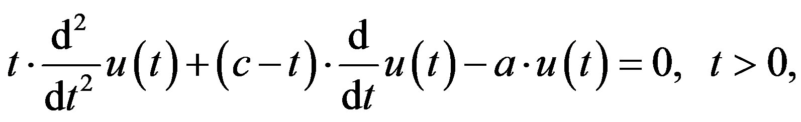
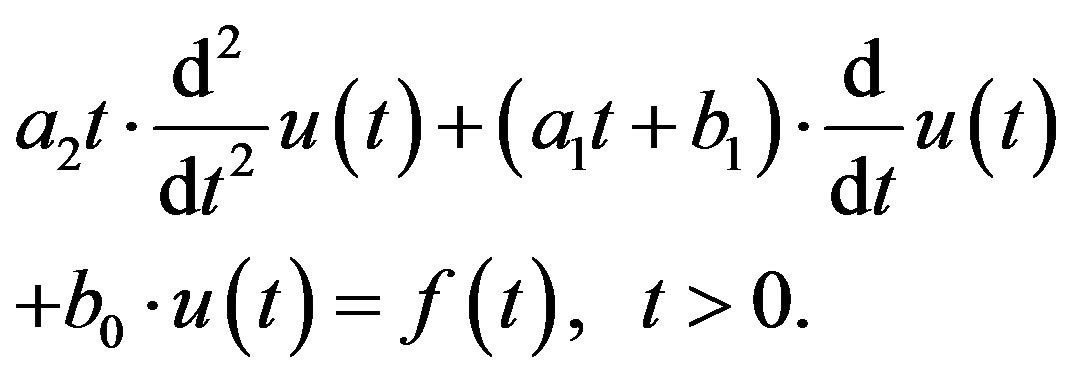
Yosida [1,2] discussed the solution of Laplace’s differential equation (DE), which is a linear DE, with coefficients which are linear functions of the variable. The DE which he takes up is
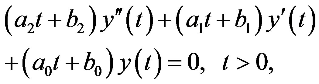 (1.1)
(1.1)
where  and
and  for
for  are constants. His discussion is based on Mikusiński’s operational calculus [3]. Yosida [1,2] gave there only one of the solutions of the DE (1.1).
In the preceding paper [4], we discussed the solution of an fractional differential equation (fDE) of the type of DE (1.1), that is given by
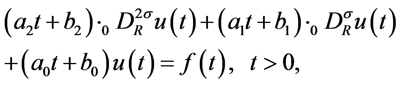 (1.2)
(1.2)
for  and
and . Here
  for
for  is the Riemann-Liouville fractional derivative (fD) defined in Section 2. We use
  to denote the set of all real numbers, and
 . When
  is equal to an integer
 ,
, . When
 , (1.2) is the inhomogeneous DE for (1.1). We use
  to denote the set of all integers, and
 ,
,  and
and
 for
for  satisfying
 .
.
We use  for
for , to denote the least integer that is not less than
 .
.
In [4], we adopt operational calculus in the framework of distribution theory developed for the solution of the fDE with constant coefficients in [5,6]. In [4], we give the recipe of obtaining the solution of the inhomogeneous equation as well as the homogeneous one, and we show how the set of two solutions of the homogeneous equation is attained.
In [4], we adopt the usual definition of the Riemann-Liouville fD, which defines  only for such a locally integrable function
  on
on  that
that
 is finite. Practically, we adopt Condition B in
[4], which is Condition IB  and
and  are expressed as a linear combination of
  for
for .
.
Here  is Heaviside’s step function, and when
  is defined on
 ,
,  is assumed to be equal to
  when
when  and to
  when
when .
.  is defined by
 (1.3)
(1.3)
for , where
  is the gamma function.
In [4], we take up Kummer’s DE as an example, which is
 (1.4)
(1.4)
where  are constants. If
 , one of the solutions given in [7,8] is
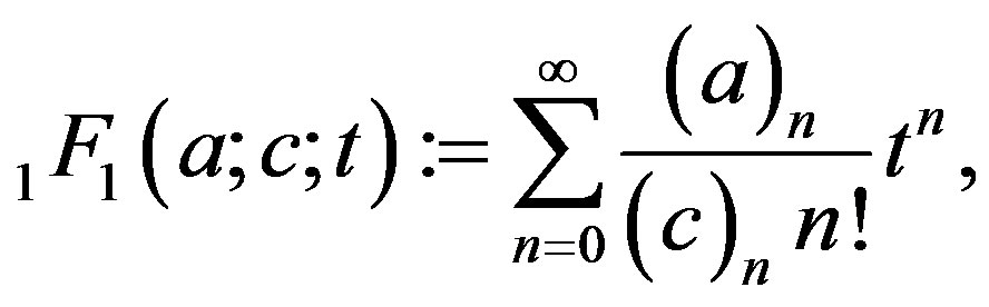 (1.5)
(1.5)
where  for
for  and
and and
and . The other solution is
 (1.6)
(1.6)
In [4], if , we obtain both of the solutions. But when
 , (1.6) does not satisfy Condition IB and we could not get it.
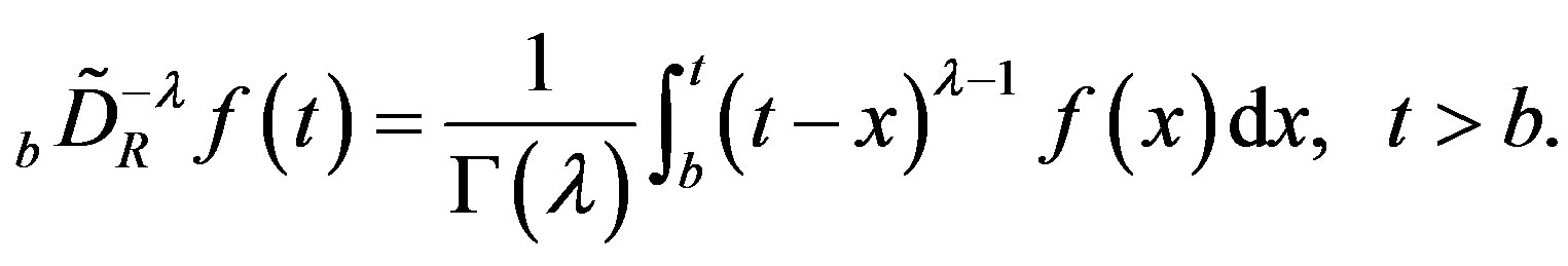
In a recent review [9], we discussed the analytic continuations of fD, where an analytic continuation of Riemann-Liouville fD,  , is such that the fD exists even for such a locally integrable function
  on
on
 that
that  diverges. In the present paper, we adopt this analytic continuation of
 .
.
In place of the above Condition IB, we now adopt the following condition.
Condition A  and
and  are expressed as a linear combination of
  for
for , where
  is a set of
  for some
 .
.
As a consequence, we can now achieve ordinary solutions for (1.2) of . For (1.4), we obtain both solutions (1.5) and (1.6) if
 .
.
It is the purpose this paper to show how the presentation in [4] should be revised, with the change of definition of fD and the replacement of Condition IB with Condition A.
In Section 2, we prepare the definition of RiemannLiouville fD and then explain how the function  and its fD in (1.2) are converted into the corresponding distribution
  and its fD in distribution theory, and also how
  is converted back into
 . After these preparation, a recipe is given to be used in solving the fDE (1.2) with the aid of operational culculus in Section 3. In this recipe, the solution is obtained only when
 and
and . When
 ,
,  is also required. An explanation of this fact is given in Appendices C and D of [4]. In Section 4, we apply the recipe to (1.2) where
  and
and , of which special one is Kummer’s DE. This is an example which Yosida [1,2] takes up. In Section 5, we apply the recipe to the fDE with
 , assuming
 .
.
For the Hermite DE with inhomogeneous term, Levine and Malek [10] showed that there exist particular solutions in the form of polynomial. In Appendices A and C, we show that such a solution exists for the DE and fDE studied in Sections 4 and 5, respectively. In Appendix B, we show how the results presented in [10] are derived from those in Appendix A.
2. Formulas
We now adopt Condition A. We then express  as follows;
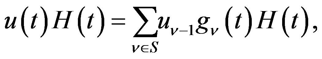 (2.1)
(2.1)
where  are constants.
Lemma 1 For ,
,
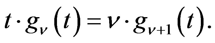 (2.2)
(2.2)
Proof By (1.3), for , we have
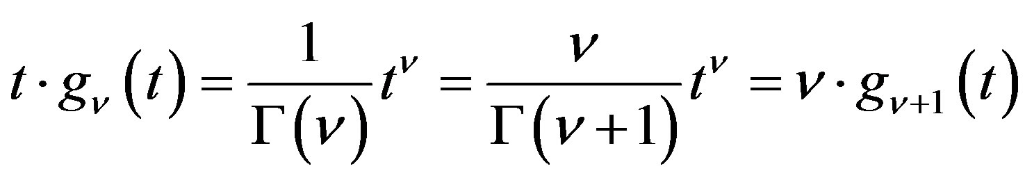 .
. 
2.1. Riemann-Liouville Fractional Integral and Derivative
Let  be locally integrable on
 . We then define the Riemann-Liouville fractional integral,
  , of order
  by
by
 (2.3)
(2.3)
We then define the Riemann-Liouville fD,  , of order
 , by
, by
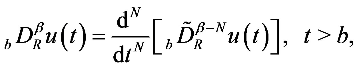 (2.4)
(2.4)
if it exists, where , and
, and  for
for .
.
For , we have
 (2.5)
(2.5)
If we assume that  takes a complex value,
  by definition (2.3) is analytic function of
  in the domain
 , and
, and  defined by (2.4) is its analytic continuation to the whole complex plane. If we assume that
  also takes a complex value,
  defined by (2.4) is an analytic function of
  in the domain
 . The analytic continuation as a function of
  was also studied. The argument is naturally concluded that (2.5) should apply for the analytic continuation, even in
  except at the points where
 ; see [9].
We now adopt this analytic continuation of  to represent
 , and hence we accept the following lemma.
Lemma 2 (2.5) holds for every ,
, .
.
By (2.1) and (2.5), we have
 . (2.6)
For  defined by (2.1), we note that
is locally integrable on .
.
2.2. Fractional Integral and Derivative of a Distribution
We consider distributions belonging to . When a function
  is locally integrable on
  and has a support bounded on the left, it belongs to
  and is called a regular distribution. The distributions in
  are called right-sided distributions.
A compact formal definition of a distribution in  and its fractional integral and derivative is given in Appendix A of [4].
Let  be a regular distribution. Then
 for
for  is also a regular distribution, and distribution
  is defined by
 (2.7)
(2.7)
Let , and let
  be such a regular distribution that
  is continuous and differentiable on
 , for every
 . Then
  is defined by
 (2.8)
(2.8)
Let ,
,  , and let
be continuous and differentiable on  for every
 . Then
 (2.9)
(2.9)
When  is a regular distribution,
  is defined for all
 .
.
Lemma 3 For , the index law:
 (2.10)
is valid for every .
.
Dirac’s delta function  is the distribution defined by
 .
.
Let  for
for  be defined by
 (2.11)
Lemma 4 If ,
,
 (2.12)
Proof By putting  in (2.7) and using (2.11) and (2.5), we obtain
By operating  to this and using (2.9) and (2.5), we obtain (2.12).
Corresponding to  expressed by (2.1), we define
  by
by
 (2.13)
Then  and
and  are expressed as
 (2.14)
where
 (2.15)
Because of (2.11), we have
 (2.16)
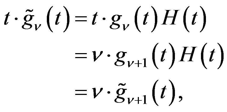
Lemma 5 Let . Then
 (2.17)
 (2.18)
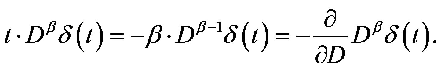
The last derivative with respect to  is taken regarding
  as a variable.
A proof of (2.17) for  is given in Appendix B of [4].
Proof When ,
,  , by Lemmas 4 and 1,
The first equality in (2.18) is obtained from (2.17) and vice versa, by using (2.11). 
The following lemma is a consequence of this lemma.
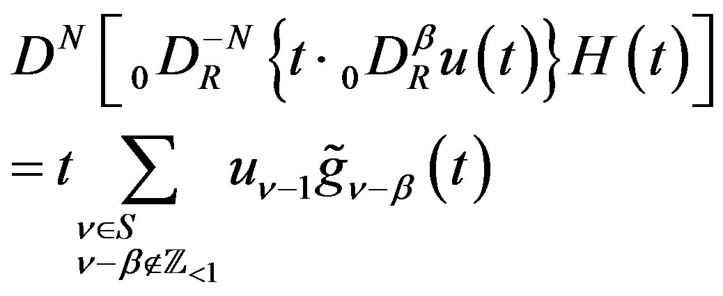
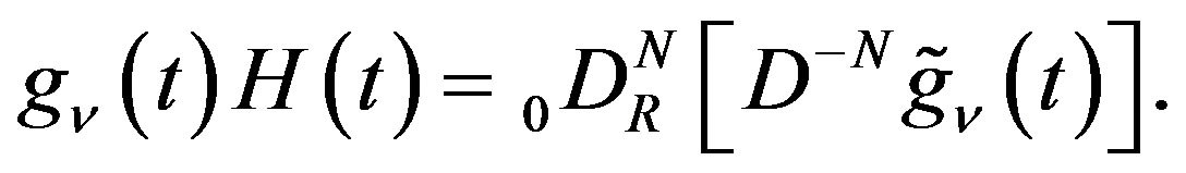
Lemma 6 Let  be expressed as a linear combination of
  for
for . Then
 (2.19)
2.3. From  to
to  and Vice Versa
Lemma 7 Let ,
,  satisfy
 . Then
 (2.20)
 (2.21)
Proof Formula (2.20) is derived by applying (2.3), (2.12) and (2.16) to the righthand. Formula (2.21) follows from (2.20) by replacing  and
and  by
by , and
, and , respectively, by using (2.2) and (2.17).
By using Lemma 7 to (2.6), we obtain
 (2.22)
 (2.23)
Lemma 8 Let ,
,  satisfy
 . Then
 (2.24)
This follows from (2.20).
Condition B  is expressed as a linear combination of
  for
for , where
  is a set of
 , for some
 .
.
When this condition is satisfied,  is expressed as (2.13) with
  replaced by
 .
.
Lemma 9 Let  satisfy Condition B. Then the corresponding
  is obtained from
 , by
, by
 (2.25)
and is expressed by (2.1) with  replaced by
 .
.
Lemma 10 Let  and
and  be given by (2.13) and (2.1), respectively. Then
  and
and  are related by
 (2.26)
 (2.27)
if  satisfies
 .
.
Proof By (2.13) and (2.16), we have
 (2.28)
Using (2.22) in the first term on the righthand side, we obtain (2.26). Multiplying (2.28) by  and noting that the first term on the righthand side is then equal to (2.23), we obtain (2.27).
3. Recipe of Solving Laplace’s DE and fDE of That Type
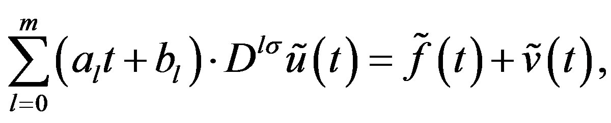
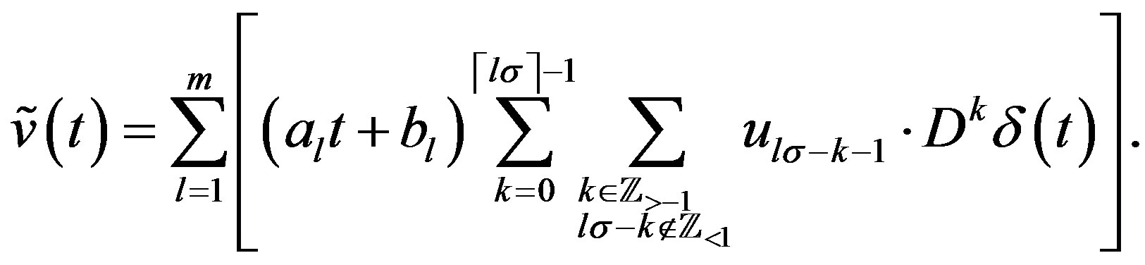
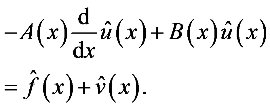
We now express the DE/fDE (1.2) to be solved, as follows:
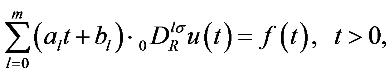 (3.1)
(3.1)
where  or
or , and
, and . In Sections 4 and 5, we study this DE for
  and this fDE for
 , respectively.
3.1. Deform to DE/fDE for Distribution
Using Lemma 10, we express (3.1) as
 (3.2)
(3.2)
where
 (3.3)
(3.3)
3.2. Solution Via Operational Calculus
By using (2.14) and (2.19), we express (3.2) as
 (3.4)
(3.4)
where
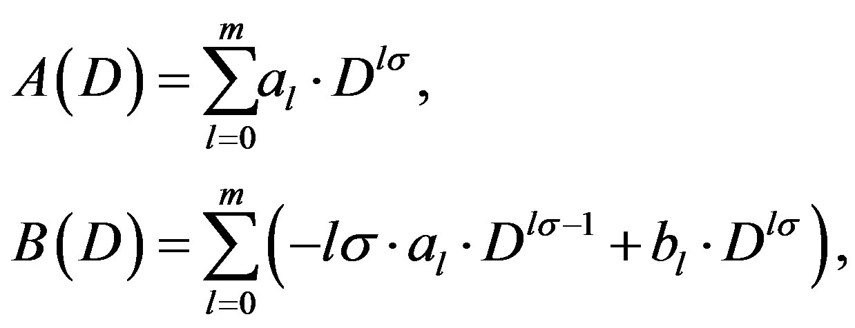 (3.5)
(3.5)
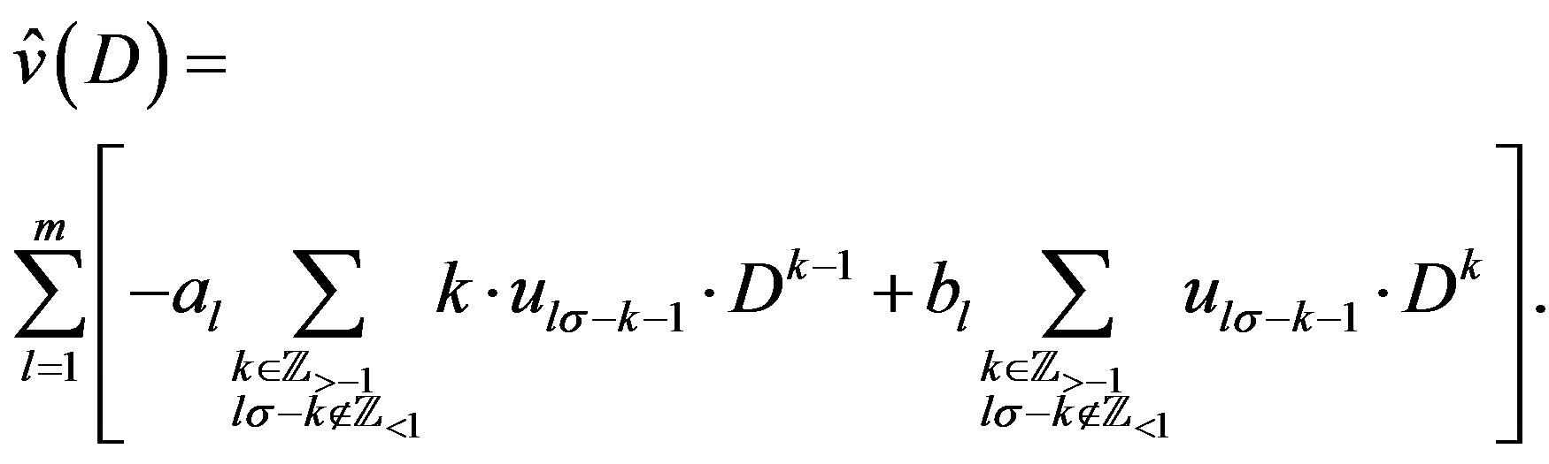 (3.6)
(3.6)
In order to solve the Equation (3.4) for
 we solve the following equation for function
  of real variable
 :
:
 (3.7)
(3.7)
Lemma 11 The complementary solution (C-solution) of equation (3.7) is given by , where
  is an arbitrary constant and
 (3.8)
(3.8)
where the integral is the indefinite integral and  is any constant.
Lemma 12 Let  be the C-solution of (3.7), and
  be the particular solution (P-solution) of (3.7), when the inhomogeneous term is
  for
for . Then
 (3.9)
(3.9)
where  is any constant.
Since  satisfies Condition A and
  is given by (3.6), the P-solution
  of (3.7) is expressed as a linear combination of
  for
for , and of
  for
for , respectively.
From the solution  of (3.7),
  is obtained by substituting
  by
by . Then we confirm that (3.4) is satisfied by that
  operated to
 .
.
3.3. Neumann Series Expansion
Finally the obtained expression of  is expanded into Neumann series [11]. Practically we expand it into the sum of terms of negative powers of D, and then we obtain the solution
  of (3.4). If the obtained
  is a linear combination of
  for
for  with some
 , then
  is the solution
  of (3.2). If it satisfies Condition B, it is converted to a solution
  of (3.1) for
 , with the aid of Lemma 9.
3.4. Recipe of Obtaining the Solution of (3.1)
1) We prepare the data:  by (2.14), and
 ,
,  and
and  by (3.5) and (3.6).
2) We obtain  by (3.8). The C-solution of (3.2) is given by
If , the C-solution of (3.1) is obtained from this with the aid of Lemma 9.
3) If  or
or , we obtain
  given by (3.9).
4) If  and
and , the solution of (3.2) is given by
 (3.10)
where  are constants. The C-solution of (3.1) is then obtained from this with the aid of Lemma 9.
5) If , the P-solution of (3.2)
is given by
where  and
and  are constants. The P-solution of (3.1) with inhomogeneous term
is obtained from this with the aid of Lemma 9.
3.5. Comments on the Recipe
In the above recipe, we first obtain the C-solution of (3.7), that is . It gives the C-solution
  of (3.4) and hence the C-solutions
  of (3.2). A C-solution
  of (3.1) is then obtained with the aid of Lemma 9.
We next obtain the P-solution  of (3.7), when the inhomogeneous part is
  for
for . As noted above, the P-solutions
  of (3.7) for
  and for
 , are expressed as a linear combination of
  for
for , and of
  for
for , respectively. The sum of the P-solutions
  of (3.7) for
  and for
  gives the P-solution
  of (3.4) and hence the P-solution
  of (3.2). The C-solution
  of (3.1) comes from the C-solution of (3.7) and the P-solution of (3.7) for
 .
.
3.6. Remarks
When we obtain  at the end of Section 3.2, we must examine whether it is compatible with Condition B. We will find that if
  for
for , the obtained
  is not acceptable. Hence we have to solve the problem, assuming that
  for all
 .
.
When  and
and , we put
 . When
 and
and , we put
 . Discussion of this problem is given in Appendices C and D of [4]. In the present case, the discussion must be read taking Condition B there to represent the present Condition B.
4. Laplace’s and Kummer’s DE
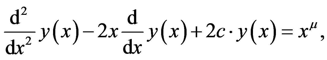
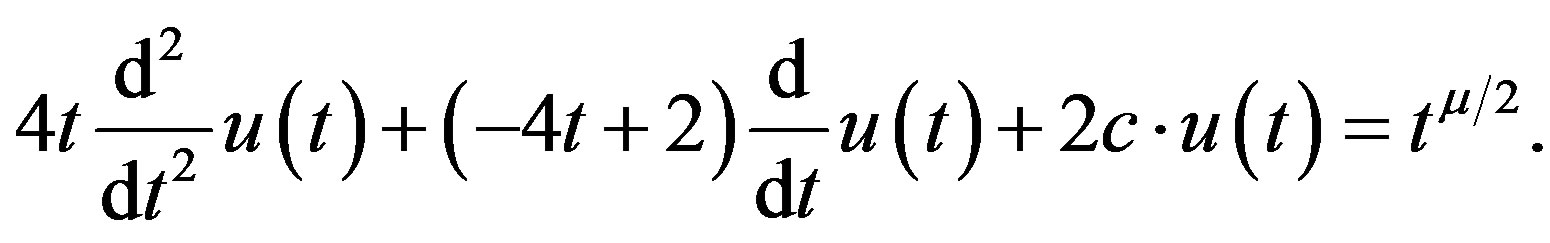
We now consider the case of σ = 1, m = 2,  , and
, and . Then (3.1) reduces to
 (4.1)
(4.1)
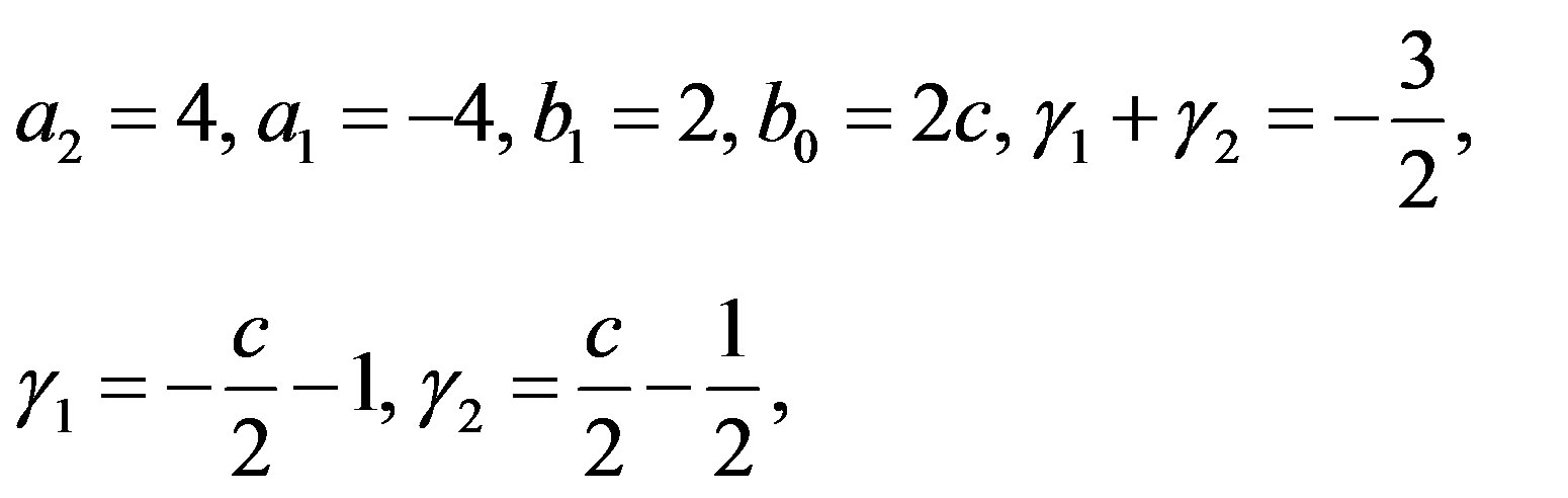
By (3.5) and (3.6),  ,
,  and
and  are
are
 (4.2)
(4.2)
 (4.3)
(4.3)
where .
.
4.1. Complementary Solution of (3.7), (3.2) and (4.1)
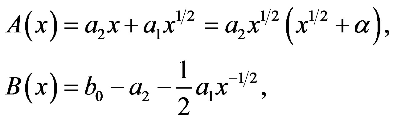
In order to obtain the C-solution  of (3.7) by using (3.8), we express
  as follows:
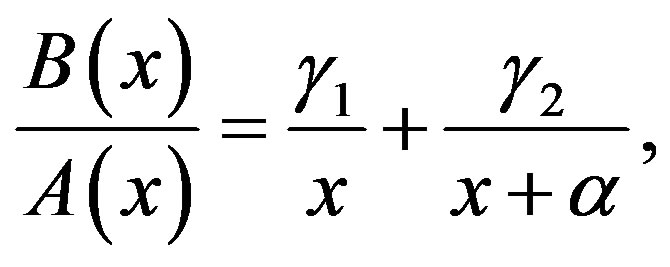 (4.4)
(4.4)
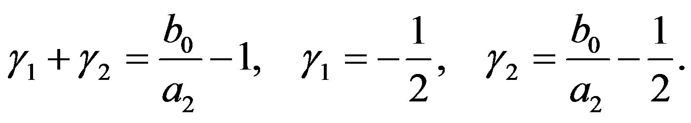
where
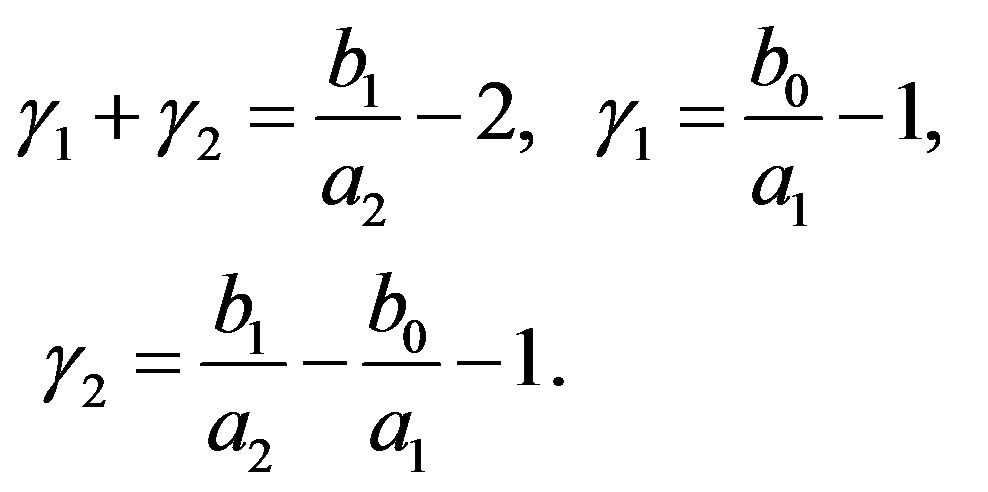 (4.5)
(4.5)
B(x) is now expressed as .
.
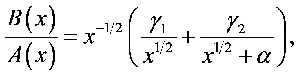
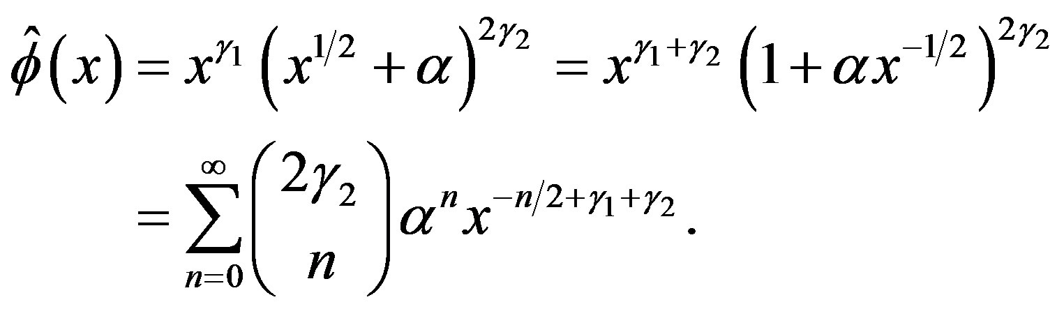
By using (3.8), we obtain
 (4.6)
(4.6)
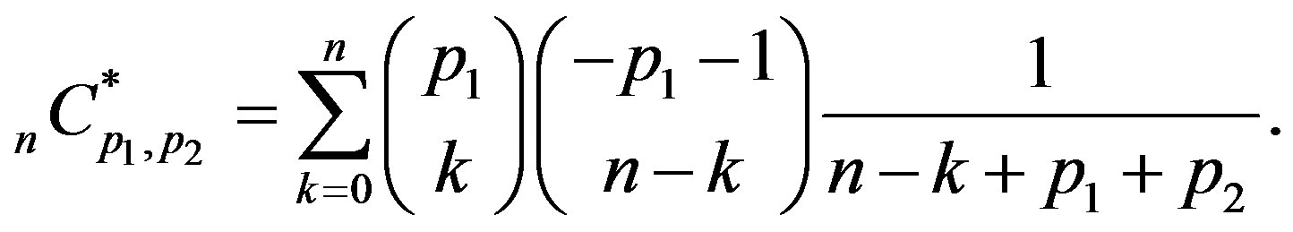
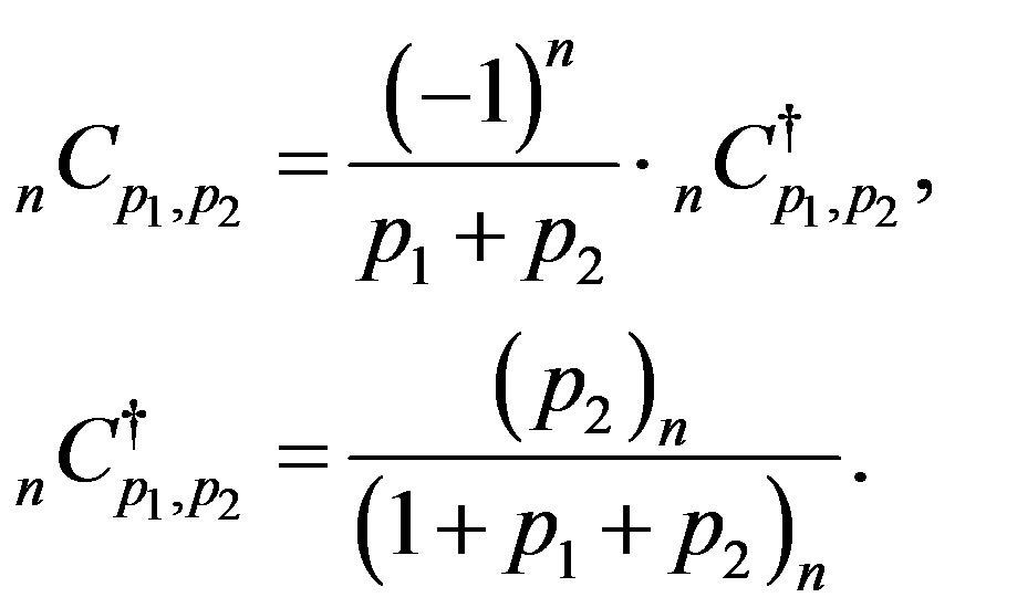
where  for
for  and
and  are the binomial coefficients.
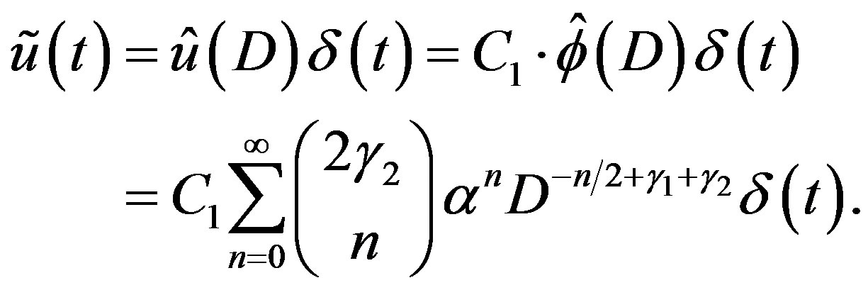
The C-solution of (3.2) is given by
 (4.7)
(4.7)
If , we obtain a C-solution of (4.1), by using Lemma 9:
 (4.8)
(4.8)
Remark 1 In Introduction, Kummer’s DE is given by (1.4). It is equal to (4.1) for ,
,  ,
,  and
and . In this case,
 (4.9)
(4.9)
We then confirm that the expression (4.8) for  agrees with (1.6), which is one of the C-solutions of Kummer’s DE given in [7,8].
4.2. Particular Solution of (3.7)
We now obtain the P-solution of (3.7), when the inhomogeneous term is equal to  for
for .
.
When the C-solution of (3.7) is , the P-solution of (3.7) is given by (3.9). By using (4.2) and (4.6), the following result is obtained in [4]:
 (4.10)
where
 (4.11)
Lemma 13 When ,
,  defined by (4.11) is expressed as
 (4.12)
This lemma is proved in [4].
4.3. Particular Solutions of (3.2) and (4.1)
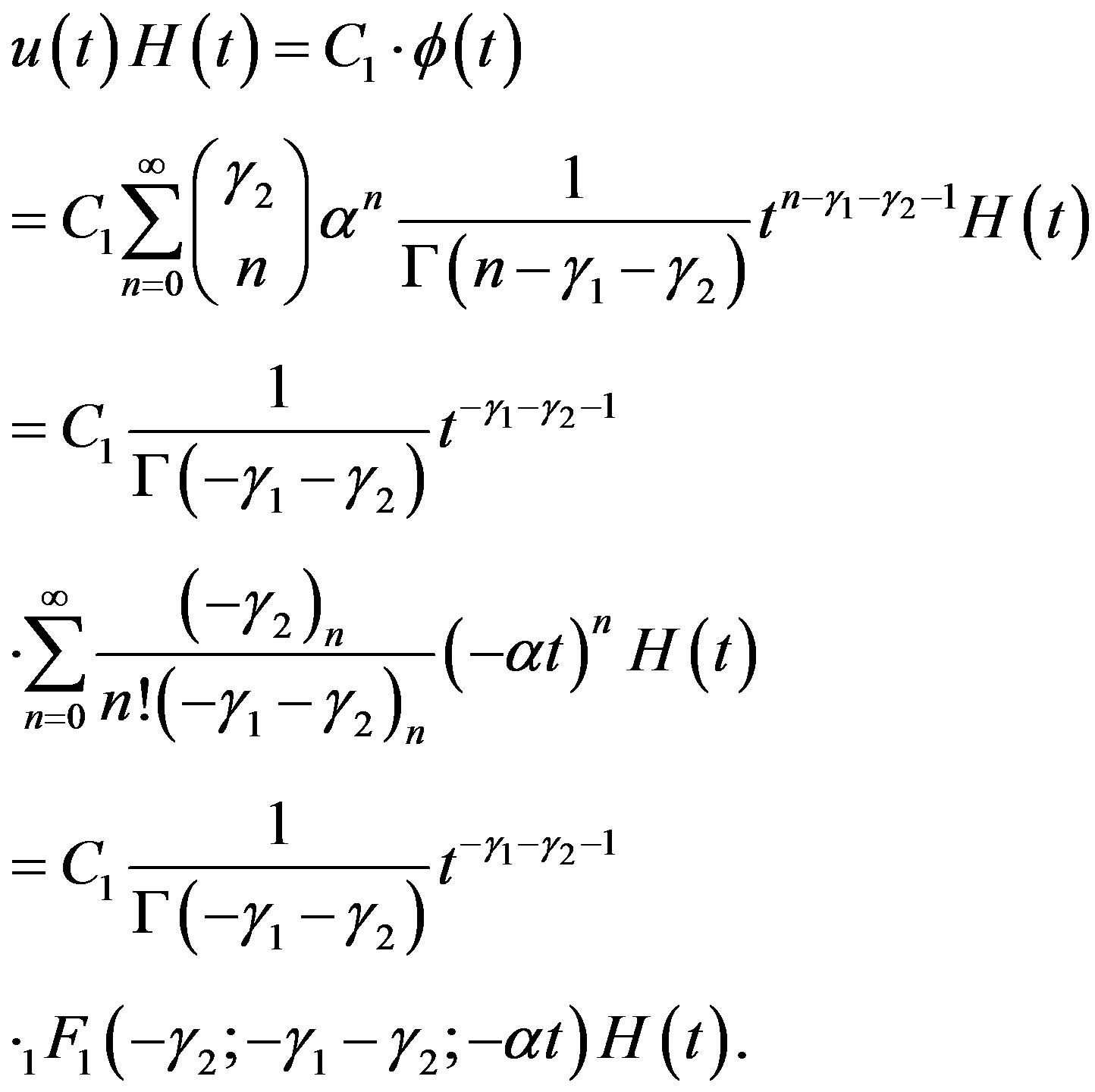
Equation (4.10) shows that if the inhomogeneous term is  for
for , the P-solution of (3.2) is given by
 (4.13)
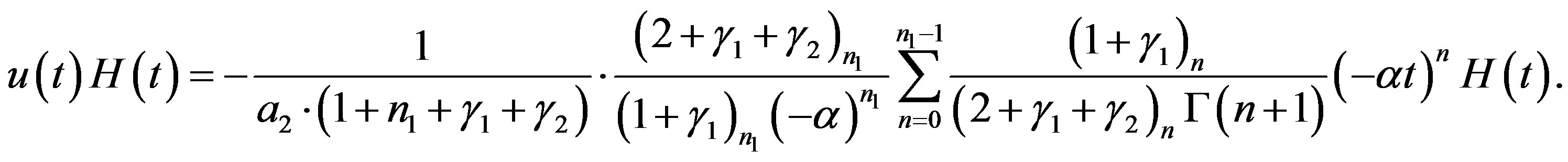
Theorem 1 Let ,
,  , and
, and . Then we have a P-solution
  of (4.1), given by
 (4.14)
where
 (4.15)
Proof Applying Lemma 9 to (4.13), we obtain
 (4.16)
By using (4.12) in (4.16), we obtain (4.14) with (4.15). 
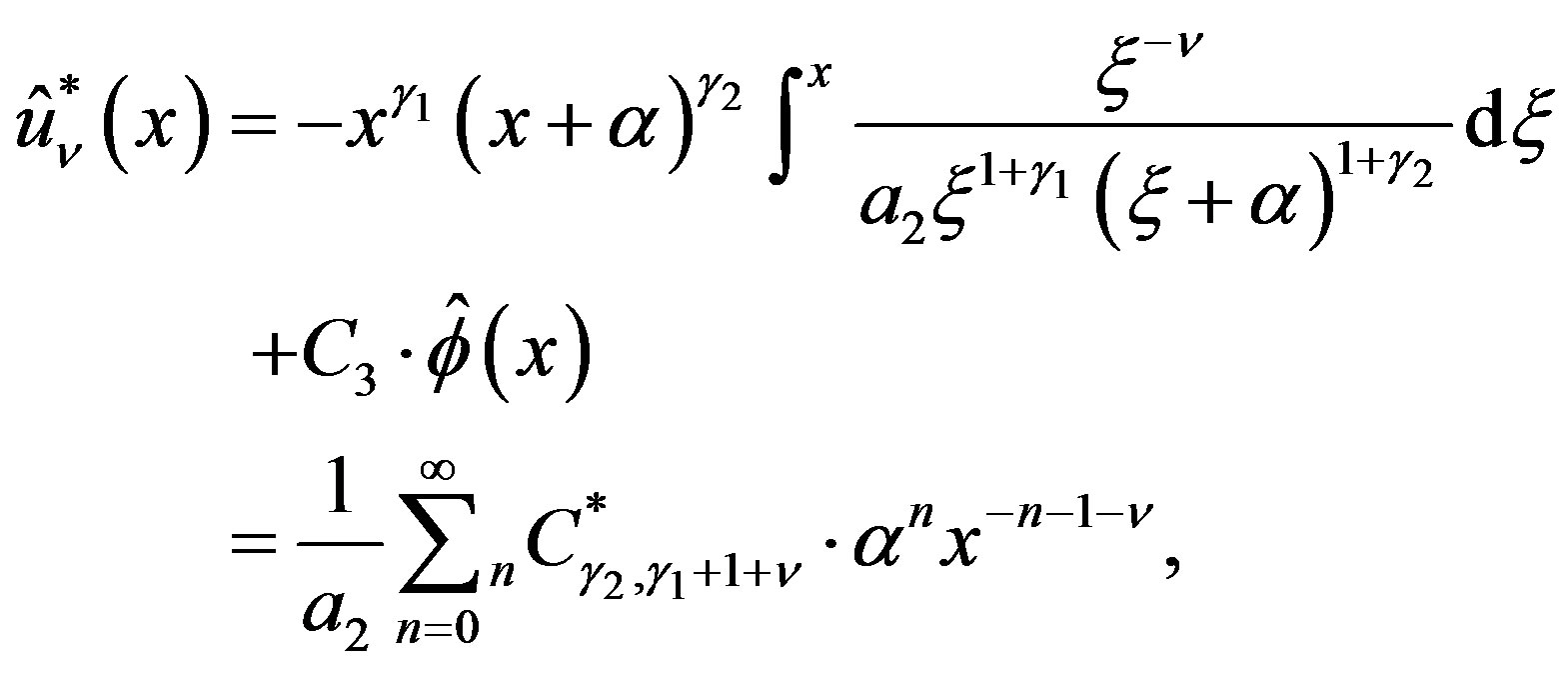
We note that  is expressed as
 (4.17)
 (4.18)
4.4. Complementary Solution of (4.1)
By (4.3) and (4.5), . When
 and
and , the P-solution of (4.7) is given by
 (4.19)
By using (4.14) for , if
, if , we obtain a C-solution of (4.1):
 (4.20)
In Section 4.1, we have (4.8), that is another C-solution of (4.1). If we compare (4.8) with (4.15), when , it can be expressed as
 (4.21)
Proposition 1 When , the complementary solution of (4.1), multiplied by
 , is given by the sum of the righthand sides of (4.8) and of (4.20), which are equal to
  and
and respectively.
Remark 2 As stated in Remark 1, for Kummer’s DE,  and
and  are given in (4.9), and
 (4.22)
We then confirm that if , the set of (4.8) and (4.20) agrees with the set of (4.5) and (4.6).
4.5. Remarks
In [10], it was shown that there exist P-solutions expressed by a polynomial for inhomogeneous Hermite’s DE, et al. We can obtain the corresponding result for Laplace’s DE. We discuss this problem in Appendix A, and then discuss the P-solution of inhomogeneous Hermite’s DE in the present formulation in Appendix B.
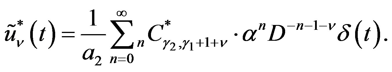
5. Solution of fDE (3.1) for 
In this section, we consider the case of ,
,  ,
,
 , and
, and Then the Equation (3.1) to be solved is
 (5.1)
(5.1)
Now (3.5) and (3.6) are expressed as
 (5.2)
(5.2)
 (5.3)
(5.3)
where .
.
5.1. Complementary Solution of (3.7)
By using (5.2),  is expressed as
 (5.4)
(5.4)
where
 (5.5)
(5.5)
By (3.8), the C-solution  of (3.7) is given by
 (5.6)
(5.6)
5.2. Complementary Solution of (3.2) and (5.1)
The C-solution of (3.2) is given by
 (5.7)
(5.7)
If , by applying Lemma 9 to this, we obtain the C-solution of (5.1):
 (5.8)
(5.8)
5.3. Particular Solution of (3.2) and (5.1)
By using the expressions of  and
and  given by (5.2) and (5.6) in (3.9), we obtain the P-solution of (3.7), when the inhomogeneous term is
  for
for :
:
 (5.9)
(5.9)
where  is defined by (4.11) and is given by
(4.12), if .
.
By using (4.12) in (5.9), we can show that if the inhomogeneous term is  for
for , the P-solution of (3.2) is
 . By applying Lemma 9 to this, we obtain the following theorem.
Theorem 2 Let ,
,  and
and  . Then we have a P-solution
of (5.1), given by
 (5.10)
where
 (5.11)
In Appendix C, discussion is given to show that there exist P-solutions in the form of polynomial for (5.1).
5.4. Complementary Solution of (5.1)
We obtain the solution  only for
 . Even though we have P-solutions of (3.2) for
 , when
  is given by (5.3) with nonzero values of
 , it does not satisfy Condition B, and does not give a solution of (5.1). Hence
  given by (5.8) is the only C-solution of (5.1).
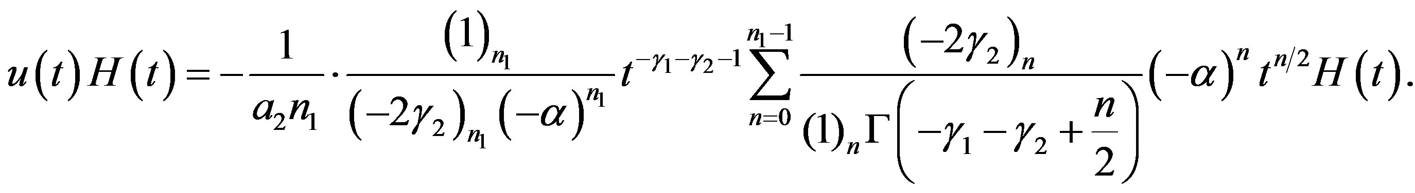
If we compare (5.8) with (5.11), we obtain the following proposition.
Proposition 2 Let . Then the C-solution of (5.1) is given by
 (5.12)
REFERENCES
- K. Yosida, “The Algebraic Derivative and Laplace’s Differential Equation,” Proceedings of the Japan Academy, Vol. 59, Ser. A, 1983, pp. 1-4.
- K. Yosida, “Operational Calculus,” Springer-Verlag, New York, 1982, Chapter VII.
- J. Mikusiński, “Operational Calculus,” Pergamon Press, London, 1959.
- T. Morita and K. Sato, “Remarks on the Solution of Laplace’s Differential Equation and Fractional Differential Equation of That Type,” Applied Mathematics, Vol. 4, No. 11A, 2013, pp. 13-21.
- T. Morita and K. Sato, “Solution of Fractional Differential Equation in Terms of Distribution Theory,” Interdisciplinary Information Sciences, Vol. 12, No. 2, 2006, pp. 71-83.
- T. Morita and K. Sato, “Neumann-Series Solution of Fractional Differential Equation,” Interdisciplinary Information Sciences, Vol. 16, No. 1, 2010, pp. 127-137.
- M. Abramowitz and I. A. Stegun, “Handbook of Mathematical Functions with Formulas, Graphs and Mathematical Tables,” Dover Publ., Inc., New York, 1972, Chapter 13.
- M. Magnus and F. Oberhettinger, “Formulas and Theorems for the Functions of Mathematical Physics,” Chelsea Publ. Co., New York, 1949, Chapter VI.
- T. Morita and K. Sato, “Liouville and Riemann-Liouville Fractional Derivatives via Contour Integrals,” Fractional Calculus and Applied Analysis, Vol. 16, No. 3, 2013, pp. 630-653.
- L. Levine and R. Maleh, “Polynomial Solutions of the Classical Equations of Hermite, Legendre and Chebyshev,” International Journal of Mathematical Education in Science and Technology, Vol. 34, 2003, pp. 95-103.
- F. Riesz and B. Sz.-Nagy, “Functional Analysis,” Dover Publ., Inc., New York, 1990, p. 146.
Appendix A: Polynomial Form of P-Solution of (4.1)
Let  and
and . Then (4.15) gives
 (A.1)
(A.1)
 (A.2)
(A.2)
where
 (A.3)
(A.3)
We obtain the following theorems from (A.2) with the aid of Proposition 1.
Theorem 3 Let ,
,  , and
, and . Then we have the polynomial form of P-solution of (4.1):
 (A.4)
(A.4)
Theorem 4 Let ,
,  ,
,  and
and  for
for . Then we have the polynomial form of P-solution of (4.1):
 (A.5)
(A.5)
Appendix B: Polynomial Form of P-Solution of Hermite DE
We now consider the inhomogeneous Hermite DE given by
 (B.1)
(B.1)
for  and
and . We put
  and
and . Then the equation for
  is given by
 (B.2)
(B.2)
This is Laplace’s DE (4.1) with parameters
 (B.3)
(B.3)
and the inhomogeneous term .
.
Theorem 5 Let ,
,  , and
, and ,
, . Then we have the polynomial form of Psolution of (B.2):
 (B.4)
(B.4)
Proof In this case,  ,
,  , and
, and
 . By Theorem 3, we obtain this result.
Theorem 6 Let ,
,  , and
, and ,
, . Then we have the polynomial form of Psolution of (B.2):
 (B.5)
(B.5)
Proof In this case,  ,
,  , and
, and . By Theorem 4, we obtain this result.
Theorem 7 Let ,
,  , and
, and ,
, . Then we have the polynomial form of Psolution of (B.2):
 (B.6)
(B.6)
Proof In this case,  ,
,  , and
, and . By Theorem 4, we obtain this result.
Theorem 8 Let ,
,  , and
, and ,
, . Then we have the polynomial form of Psolution of (B.2):
 (B.7)
(B.7)
Proof In this case,  ,
,  , and
, and . By Theorem 3, we obtain this result.
Remark 3 We confirm that Theorems 7 and 5, respectively, agree with Theorems 1 and 2 in [10].
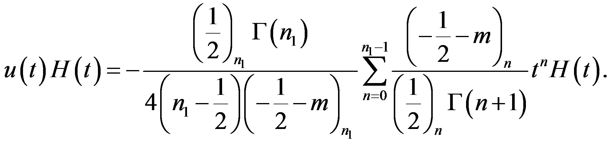
Appendix C: Polynomial Form of P-Solution of (5.1)
Let  and
and . Then (5.11) gives
 (C.1)
(C.1)
 (C.2)
(C.2)
where
 (C.3)
(C.3)
We obtain the following theorem from (C.2) with the aid of Proposition 2.
Theorem 9 Let ,
,  ,
,  and
and  for
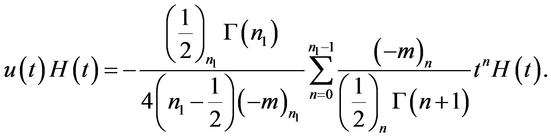
for . Then we have the polynomial form of P-solution of (5.1):
 (C.4)
(C.4)