ABSTRACT

This paper examines general variance-covariance structures for the specific effects and the overall error term in a twoway random effects (RE) model. So far panel data literature has only considered these general structures in a one-way model and followed the approach of a Cholesky-type transformation to bring the model back to a “classical” one-way RE case. In this note, we first show that in a two-way setting it is impossible to find a Cholesky-type transformation when the error components have a general variance-covariance structure (which includes autocorrelation). Then we propose solutions for this general case using the spectral decomposition of the variance components and give a general transformation leading to a block-diagonal structure which can be easily handled. The results are obtained under some general conditions on the matrices involved which are satisfied by most commonly used structures. Thus our results provide a general framework for introducing new variance-covariance structures in a panel data model. We compare our results with [1] and [2] highlighting similarities and differences.

1. Introduction

Panel data models are often characterised by a three component error structure consisting of an individual (time invariant) specific effect, a time specific (individual invariant) effect and an overall idiosyncratic error term varying in both the individual and time dimensions. This leads to a corresponding three component variance covariance structure for the combined error term of the model. Due to the potentially large dimension of this variance covariance matrix, its inverse is usually calculated using matrix decomposition results. In a seminal paper [3] derived the spectral decomposition of the variance-covariance matrix of a two-way (and a one-way) random effects (error component-EC) model when all the components are assumed to be i.i.d. and independent two by two.

Several works have extended Nerlove’s result when non-i.i.d. structures are assumed for the error terms, namely, an MA(1) for the overall error term in [4], an AR(1) structure for the overall error term in [5], an ARMA structure for the overall error term in [6-8]. All these studies consider a one-way EC i.e. only individual effect in addition to the overall error term, and apply a first-stage Cholesky-type transformation in order to get back to a “classical” one-way EC setting in which both the individual effect and the idiosyncratic error are i.i.d. after the transformation. Once we get back to the “classical” setting, we can apply Nerlove’s spectral decomposition for implementing the GLS procedure. Thus, all the studies so far have employed a combination of a first stage Cholesky and a second stage spectral decomposition.

In this note, we first show that the Cholesky-spectral combination approach adopted by all the above-mentioned articles is not possible in a two-way setting and there exists no transformation that will get us back to a “classical” EC structure. Then we propose a solution to the problem through a different first stage transformation based on a new spectral decomposition result which we present and prove. This new result is derived for two way EC models with general variance-covariance structures for all the error components. Our first stage transformation does not yield a classical two-way EC but a one-way EC with heteroscedastic errors and we show that the spectral decomposition and hence the determinant of the variance covariance matrix of the transformed errors is easy to obtain, thus making GLSand Maximum Likelihood-type procedures operational.

A recent article [1] provides a solution for the inverse and determinant of some general variance covariance structures in panel data models including a general one-way EC setting with a variance covariance matrix of the form 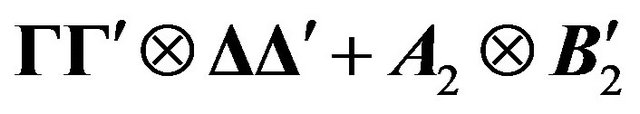where is a matrix of full column rank, is a matrix of full column rank, A₂ and B₂ are positive definite matrices of order and respectively. They showed that a two-way EC of the form 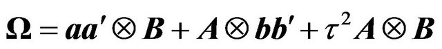, where a is a T-vector, b is a N-vector, A is, and B is, is a special case of the above general one-way EC. However, the authors add that if one were to generalise the traditional three component structure, namely 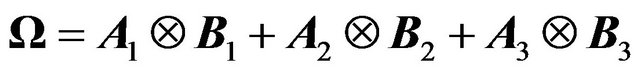, where all the first matrices of the Kronecker products are of order and the second ones, then “the inverse is not easily computable in general”. The above general Kronecker structure is precisely what we consider in our note and we propose a general two-stage transformation for calculating its inverse and determinant under some conditions¹ Thus our result represents a natural follow up to the note by [1]. Our note partially validates their conjecture as our first stage spectral transformation yields a two component heteroscedastic structure and we do bring the model to a two component variance structure at an intermediate stage. However, we say only “partially” as we cannot rewrite our original variance matrix as a two component variance structure but apply a transformation to convert a general three component variance structure into a two component one.

Another more recent study [2] presents a general approach for a two-way EC under double autocorrelation in both the time effect and the idiosyncratic error. They propose a transformation based on a mixture of Cholesky and spectral decompositions as a first stage (what we call a “hybrid” transformation in this note), and a spectral decomposition as a second stage. In our note, we use our methodology to extend their approach to more general structures at the cross-sectional level. We derive the spectral decomposition as well as the determinant of the resulting variance-covariance matrix whereas [2] only derives the inverse of the transformed variance-covariance matrix.

The paper is organised as follows. Section 2 shows why Cholesky-type transformations do not work in the two-way EC model. In Section 3 we derive the new “spectral-spectral” combination result for general structures of variance-covariance matrices. The new transformation is obtained under some conditions that are satisfied for most of the structures usually encountered in a panel data setting. Section 4 takes up some of these commonly used structures and describes how a solution can be found for these structures using our new decomposition result. Section 5 presents a new transformation along the lines of [2]. Finally, we conclude by pointing out some interesting aspects of our approach that may be worth investigating further.

2. On the Impossibility of Cholesky Decomposition in a Two-Way Error Component Context

Consider the following panel data model:

(1)

where

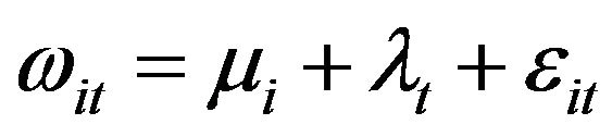
with denoting the individual specific random effect, denoting the time specific random effect, the overall idiosyncratic error term, and where is a vector of coefficients including the intercept, i and t denote the individual and the time period respectively, is a vector of observations on k strictly exogenous explanatory variables. is assumed to follow a stationary process independent over, and parameterised by a vector. Writing

,

let us assume that:

where is any non-iid variance covariance structure and the disturbance components are independent two by two. Under these assumptions, the variance-covariance matrix of the linear model can be expressed as follows:

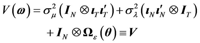(2)

In the case of a one-way EC model, the structure typically proposed in the literature for is an autocorrelated structure and a Cholesky decomposition is used to get back to a “classical” one-way EC setting. In the following lemma, we establish that in a two-way EC model it is impossible to find a Cholesky decomposition that diagonalises and gets us back to a “classical” setting. A solution to this problem is proposed in the next section.

Lemma 1. Let be a transformation matrix, where is matrix such that with. Then, there is no matrix with the above-mentioned properties that allows us to get back to a classical two-way EC model.

Proof: See Appendix A.

3. Spectral Decompositions, an Alternative

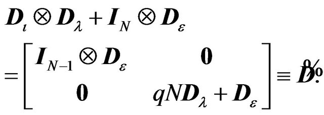
This section shows that two-stage spectral decompositions can be applied to solve the problem of an analytical inverse of V for the general variance-covariance structure (2) presented in the previous section. Before deriving the main result in the form of a theorem, we illustrate our idea in the case of a two-way EC model with autocorrelation in the overall error term, a case that may be commonly encountered in practice (for which there is no explicit solution so far).

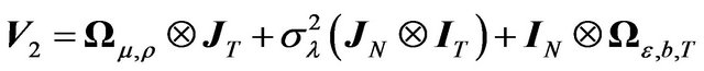
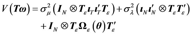
Assume that we are dealing with a panel data model with the following variance-covariance matrix (EC with MA structure for the idiosyncratic error):

(3)

where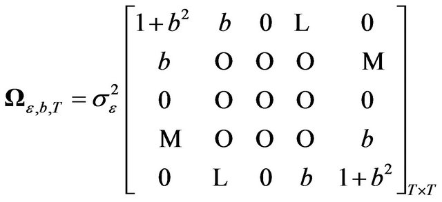

As the inverse of the above variance-covariance matrix is rather difficult to compute, if we want to apply a GLS or Maximum Likelihood procedure we need to find a transformation which will yield a variance-covariance matrix with a tractable inverse. In Section 2, we proved that it was not possible to get to the classical structure through the Cholesky decomposition. Nor is it possible to rewrite the model as a one-way EC structure. Here we show that by using the spectral decomposition, we can provide an explicit transformation that allows us to get to a model with a variance-covariance matrix that is easy to handle.

First we note that [9] has given the orthogonal matrix such that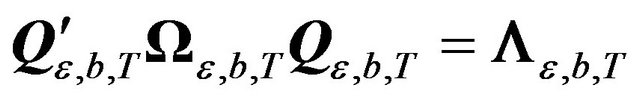, where

, is the matrix of eigenvalues of

, with. The t-th column of is given by:

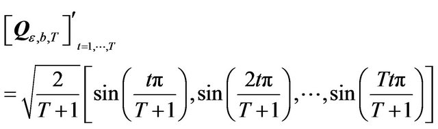(4)

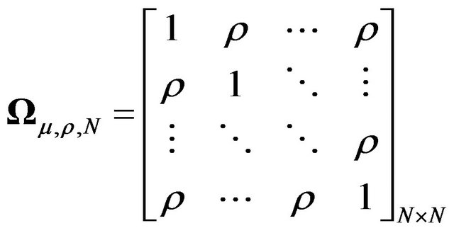
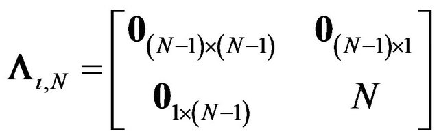
Next we derive another result (Lemma 2 below) which gives the diagonalisation of a unit matrix and shows that the same orthogonal matrix also diagonalises an equicorrelation matrix as well. This can be particularly useful in panel data models with both individual and time specific effects. In fact, one of the main problems for getting the spectral decomposition of the full variance-covariance matrix in the presence of a time effect is the cross-sectional dependence induced by the latter. Indeed, in the presence of a time effect we lose the block-diagonal structure which is found in one-way models. This lemma is useful as it allows us to obtain a transformation leading to a block-diagonal structure.

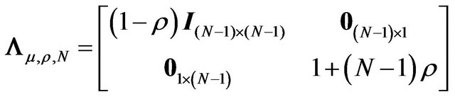
Lemma 2. Let be a vector of ones. Let and²

.

Then the same matrix diagonalises both and i.e.

where represents the orthogonal matrix of eigenvectors of both and (its expression is given in the lemma’s proof in the Appendix), and and represent the matrices of eigenvalues of and respectively.

Proof: See Appendix A.

Now combining [9]’s result and Lemma 2, we can give a transformation, which when applied to (3) will lead to a block-diagonal structure whose spectral decomposition is easily obtained (see Theorem 1 and Special Case 1). Thus GLS and ML methods become much easier to operationalise in presence of complex variance covariance structures.

The method presented above fits in a more general approach that provides a way out for obtaining the inverse of any general variance-covariance structure for the specific effects as well as the idiosyncratic error in a two-way EC setting. We derive the solution under certain assumptions which may seem restrictive at first sight but which we show to be satisfied by many general structures frequently found in the literature. In fact we also show that this theorem enables us to introduce some new and possibly relevant structures in panel data models.

Let us now consider general processes for and such that and. In other words we have individual (cross-sectional) dependence through, cross-sectional dependence and time dependence through and time dependence in.

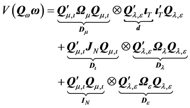
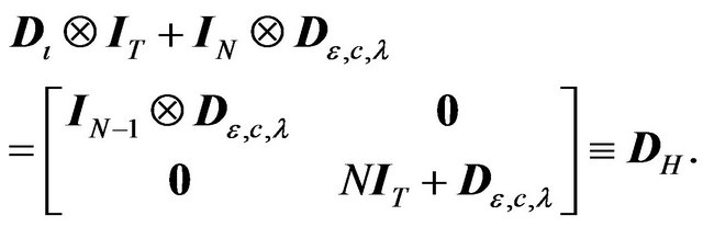
Theorem 1. Given a general variance covariance structure

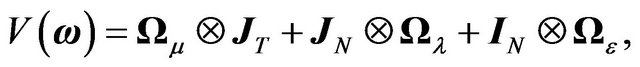
where, if

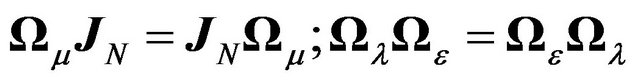(5)

then the following results hold³:

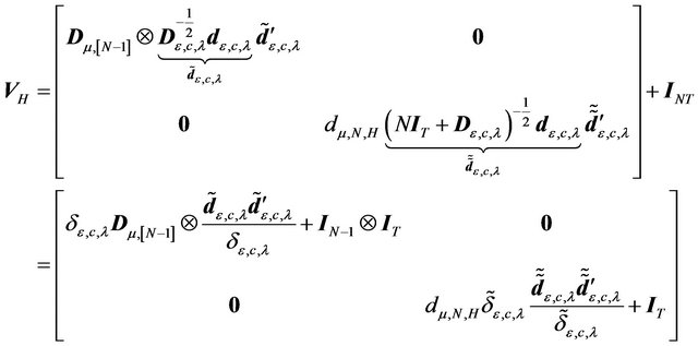
1) There exists a transformation matrix given by 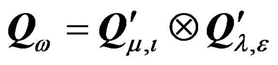such that:

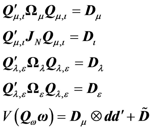(6)

where, and are orthogonal matrices, , and are diagonal matrices.

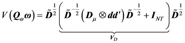
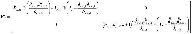
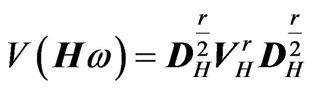
2) The spectral decomposition of the transformed variance-covariance matrix is given by:

(7)

where, is the i-th element of the diagonal matrix, , ,

and.

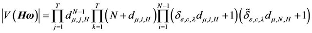
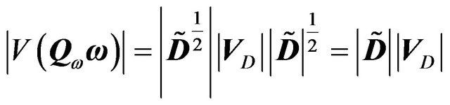
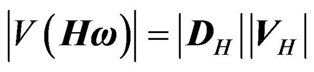
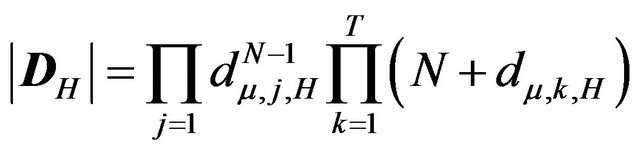
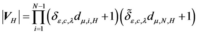
3) The determinant of the transformed variance-covariance matrix can be written as:

(8)

Proof: See Appendix B.

Remarks:

1) By assuming variance-covariance matrices of a general form for the three components in the random effects model, denoted as and, we go further than any other article that has dealt with finding appropriate transformations for non i.i.d. error structures in a panel data framework. All explicit transformations that exist in the literature are given for

or and issued from an AR(1)

and/or MA(1) process. All these features can be seen as special cases of the result stated in Theorem 1 (see Section 4).

2) Our results are derived under the double commutativity constraint (5). Though this condition looks rather restrictive, it turns out to be quite general in the panel data framework. In fact, not only all the structures studied so far in the panel econometric literature satisfy this condition but also there are other possibly interesting structures which have not yet been considered that can be included in this setting. One such structure is equicorrelation which can be particularly relevant for individual effects in certain empirical contexts. It can even be modified to reflect block dependence among individuals (correlation within clusters).

3) We show different ways of taking cross-sectional dependence into account, i.e., through and/or. The presence of the time effect is already a source of cross-sectional dependence in our model and it can be further generalised to have a fuller variance-covariance structure through. This feature can be linked to the more recent strand of literature that deals with crosssectional dependence through factor analysis.

4) Although our result is general, it may present some operational difficulties. Our transformation matrix requires the knowledge of eigenvectors and eigenvalues of the different matrices involved and it may be cumbersome to actually determine these for some structures. Unlike the MA case that we saw earlier, in the case of an AR structure for or, there are no general analytical expressions available for the eigenvectors of the resulting variance covariance matrix for any dimension T. These expressions crucially depend on the size of T. Plus there is no recursive way of finding the roots of characteristic polynomials of size T + 1 given those of size T and one has to calculate them separately for each T. These are practical obstacles to be overcome before implementing our transformation. In spite of this, we believe that our transformation is highly useful as it definitely reduces the size of the problem in all circumstances i.e. instead of finding the eigenvalues/eigenvectors of a matrix of size NT (i.e. of the full variance-covariance matrix of the model), one only needs to find them for a matrix of size T (i.e. of the AR structure over just the time dimension). In the worst case scenario, one can compute these eigenvalues and eigenvectors numerically in the first stage.

4. Some Special Cases

In this section we will examine some special cases that are commonly used for one way models and show how our result enables to extend them to the two-way case and obtain the spectral decomposition of the variance covariance matrix of the model in a rather straightforward manner. In addition, we also introduce some new structures that have not been considered so far in this context.

1) Independent’s, independent’s, and MA(1)’s with the same parameter b for all i’s. In other words and of an MA(1) process. This is the case that we already considered in the beginning of Section 3.

One can easily verify that the commutativity condition is satisfied in this case i.e. and ⁴.

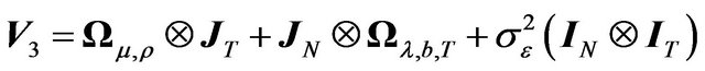
Then, the variance-covariance of the whole model writes:

(9)

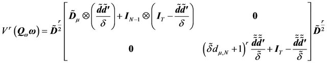
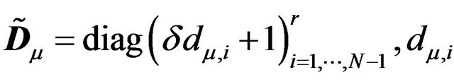
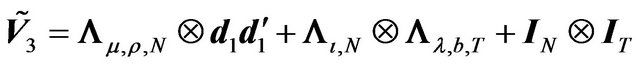
Using Theorem 1, the transformation to be applied to get a block diagonal structure is given by , with given in the Appendix and the matrix of eigenvectors of previously defined. Note that this transformation does not depend on any nuisance parameter, so it can be applied as a first stage transformation without any prior estimation. The variance-covariance matrix of the transformed error, then becomes:

(10)

with.

One can easily see that can be written in the form denoting as and the diagonal matrix as. Then the spectral decomposition of can be easily computed using the result in point 2 of Theorem 1.

2) Equicorrelated’s, independent’s, and MA(1)’s with the same parameter b for all i’s. In other words, and.

(11)

Here one can use the same transformation as in the previous point (due to Lemma 2), i.e.,. The corresponding transformed variance-covariance matrix is:

(12)

As in case 1, the spectral decomposition of the transformed variance-covariance matrix can be explicitly computed using the result in point 2 of Theorem 1 denoting as and the diagonal matrix as.

Note that the transformation for the above 2 cases does not exist in the literature. It is the first time, to our knowledge, that one can deal with cross-sectional dependence and autocorrelated errors over time in the same transformation in panel data models.

3) Equicorrelated’s, MA(1)’s, and independent’s. In other words, and .

This case is symmetric to the previous one and hence, the transformation remains the same, , the original variance-covariance being:

(13)

The variance-covariance matrix of the transformed model is:

(14)

Once again noting that the first term of is of the form and the second plus the third term is a diagonal matrix of the form, one gets the spectral decomposition of from Theorem 1.

4) Equicorrelated’s, equicorrelated’s, and equicorrelated’s. That is and.

Here we assume both cross-sectional and time equicorrelation. The transformation matrix is given by . The original variance-covariance matrix is:

(15)

and the transformed variance-covariance matrix is:

(16)

The spectral decomposition of follows from point 2, Theorem 1, as in the above cases.

5) Equicorrelated or i.i.d’s, i.i.d.’s and AR(1)’s.

Referring to our Remark 4 of Section 3, the eigenvectors of an AR(1) variance covariance matrix are different for different T’s and cumbersome to calculate. Although we have them for T = 5 for example, we do not pre-  sent them here as the expressions of the eigenvectors  are indeed long. One can also calculate them numerically. Once the first stage decomposition is obtained (perhaps numerically for the third AR component), the procedure in Theorem 1 can be implemented as in the above cases.

5. Extension to “Hybrid” Transformations

In spite of the fact that the commutativity constraint is verified in many panel data models of practical relevance, one could argue that it is stringent and may exclude some potentially important situations. For instance, assume that the researcher expects to have an autocorrelated process not only in the idiosyncratic error but also in the time effect. In general, the variance-covariance matrices of the two autocorrelated processes do not commute. [2] proposes a 3-stage transformation that circumvents the double autocorrelation problem. They successively apply the Cholesky and the spectral transformations to obtain a simpler structure for which they are able to give the inverse. Thus their first two stages are equivalent to our first stage in the sense that after two transformations they provide a way to calculate the inverse of the resulting variance-covariance matrix. However, they do not provide the spectral decomposition of the Cholesky transformed variance-covariance matrix in the first stage as it cannot be explicitly derived.

In this section we examine these more general cases and give appropriate transformations based on our previous results. These transformations are characterised by a mixture of Cholesky and spectral decompositions (what we call “hybrid” transformations) in the first stage and a spectral decomposition in the second stage. The following theorem provides a new transformation in this general setting that allows us to obtain the spectral decomposition of the resulting variance-covariance matrix.

Theorem 2. Given a general variance-covariance structure

if

(17)

then the following results hold:

1) There exists a transformation matrix of the form such that:

(18)

where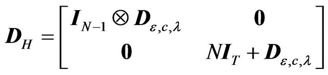, and are orthogonal matrices, , and and are diagonal matrices.

2) The spectral decomposition of the transformed variance-covariance matrix is given by:

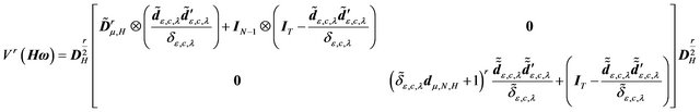(19)

where, ,

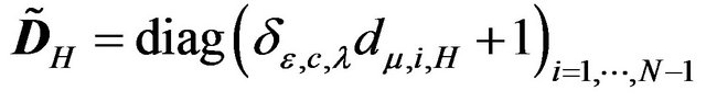
is the i-th element of the diagonal matrix,

, ,

and.

3) The determinant of the transformed variance-covariance matrix is given by:

(20)

Proof: See Appendix C.

Remarks:

1) Note that Theorem 2 considers a slightly more general structure than [2] by introducing cross-sectional dependence through in addition to that induced by the time effect.

2) The transformations given in point 1 of the theorem are called “hybrid” since they use both spectral, and, and Cholesky, , decompositions in the first stage in order to arrive at a tractable variance-covariance matrix.

3) These transformations are more general than those of Theorem 1 in the sense that they can handle more complex structures in and, in particular autocorrelation of the AR type. However, the problem of finding such transformations becomes even more difficult than in Section 3. Indeed, even if we have an idea of the Cholesky decomposition of the variance-covariance matrix of a particular stochastic process, say, such knowledge is not, in general, informative for the spectral decomposition of the variance-covariance matrix of another stochastic process, , nor for a linear transformation of the latter,. Yet, we require all these decompositions to implement the procedure.

4) The results of this section are only theoretical as we cannot provide any explicit transformation, especially in the first stage, as mentioned above. However, our earlier Theorem 1 provides an explicit solution under the commutativity constraint.

5) We still have the commutativity constraint between and in our case that extends [2]’s model to cover general variance covariance structures at the crosssectional level⁵. We conjecture that in the two-way EC this is the maximum generality that one can afford in order to get back to a heteroscedastic one-way case after the first transformation.

6. Concluding Remarks

In this paper, we examine general variance-covariance structures for the specific effects and the overall error term in a two-way error component model. We show the limitations of Cholesky-type transformations and propose a different approach, based on spectral decomposition, for dealing with time and cross-sectional dependence. Our transformation can be applied to any general variance-covariance setting, under the commutativity constraint, and we show how this transformation works in many interesting special cases. We also connect our result to [1] and their conjecture for a two-way EC which seems to be verified albeit only after an initial transformation.

As our transformation is based on eigenvalues and eigenvectors of the variance-covariance matrix of the combined disturbance term, we believe that it is strongly linked to the more recent approach of taking cross-sectional dependence into account by means of factor models. We conjecture that our approach is equivalent to the factor approach under some assumptions and we hope to investigate the link between these two approaches in the future.

Finally, we show how the result derived in [2] for the double autocorrelation structure can be extended to cover more general structures at the cross-sectional level using our method. We provide the spectral decomposition as well as the determinant of the variance-covariance matrix of the transformed model.

REFERENCES

Appendix A

Proof of Lemma 1. It is straightforward that,

(21)

In order to get back to a classical EC structure we would need two conditions:

1)

2)

However, condition 1 implies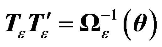. This in turn implies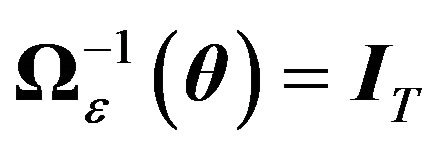. Hence the only matrix that satisfies both conditions in a two-EC is the identity matrix meaning i.i.d. errors. In this case there is no need for implementing any transformation since we are already in the classical two-way-EC case⁶.     

Proof of Lemma 2.

1) Diagonalization of

Since is symmetric, there exists an orthogonal matrix, , such that, where, the matrix of eigenvalues, is

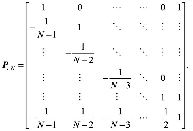
It can be easily verified that the solution for is given by with

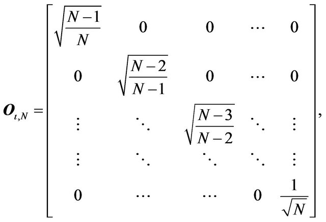
2) Diagonalization of

Same reasoning as in the previous point. is symmetric, therefore there exists an orthogonal matrix such that where, the matrix of eigenvalues, is

Direct calculation shows that of point 1 satisfies the above condition.                        

Appendix B

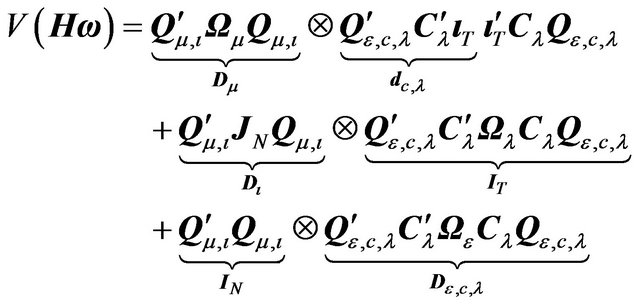
Proof of Theorem 1. The variance-covariance of the transformed error term can be written as:

(22)

Proof of point 1.

From Lemma 2 we hav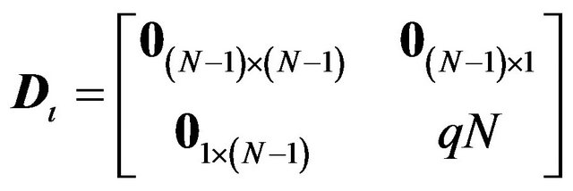e where. Hence,

This completes the proof of the first point.

Proof of point 2.

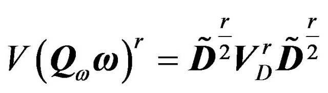
(23)

where

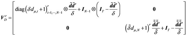
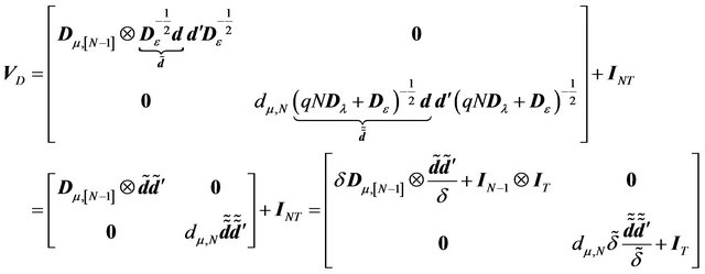(24)

with. V_D is a block diagonal matrix. Hence we can compute the spectral decomposition for each block and this will give rise to the spectral decomposition of the whole matrix. For the first blocks, we have:

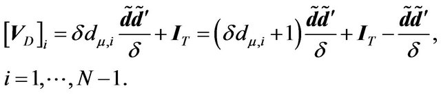(25)

and similarly for

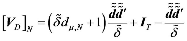
As and are idempotent, orthogonal to each other and their sum is equal to the identity matrix, the last two expressions give the spectral decompositions for each block with and 1 being the eigenvalues for blocks, and and 1 the eigenvalues for block N. Hence,

(26)

Therefore we have

(27)

Proof of point 3.

(28)

where

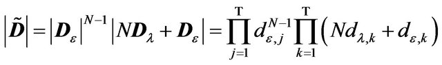(29)

For, we know that the determinant of a blockdiagonal matrix is equal to the product of the determinant of each block. Since the eigenvalues for each block are given in point 2 (spectral decomposition), the determinant of each block is equal to the product of the eigenvalues. Hence,

(30)

This completes the proof of Theorem 1.

Appendix C

Proof of Theorem 2. The variance-covariance of the transformed error term is:

(31)

Proof of point 1.

As in point 1 of Theorem 1 we have

This completes the proof of point 1.

Proof of point 2.

We proceed in the same way as in point 2 of Theorem 1.

(32)

(33)

Applying the same argument as in the previous theorem, we get:

(34)

Hence,

(35)

Proof of point 3.

(36)

where

and

This completes the proof of Theorem 2.

NOTES

¹We show that these conditions are satisfied in almost all usually assumed structures and these conditions do not imply a rewriting of the three component variance matrix as a two component one. Thus we do go beyond a two component structure.

²Note that given in this lemma represents the variance-covariance matrix of an equicorrelated error structure.

³We will come back to the commutativity condition in a remark following the theorem (see Remark 2).

⁴All the special cases discussed below satisfy this condition and hence we will not mention it each time.

⁵In their model and hence this condition is automatically satisfied.

⁶One can show that the only possibility that a Cholesky type transformation will allow us to get back to a classical EC will be when λ_t and ε_it follow the same stochastic process. As this hypothesis is very stringent, one needs to find new transformations in the general case.

REFERENCES

- J. R. Magnus and C. Muris, “Specification of Variance Matrices for Panel Data Models,” Econometric Theory, Vol. 26, No. 1, 2010, pp. 301-310. doi:10.1017/S0266466609090756
- J. M. B. Brou, E. Kouassi and K. O. Kymn, “Double Autocorrelation in Two Way Error Component Models,” Open Journal of Statistics, Vol. 1, No. 3, 2011, pp. 185- 198. doi:10.4236/ojs.2011.13022
- M. Nerlove, “A Note on Error Components Models,” Econometrica, Vol. 39, No. 2, 1971, pp. 383-396. doi:10.2307/1913351
- P. Balestra, “A Note on the Exact Transformation Associated with the First-Order Moving Average Process,” Journal of Econometrics, Vol. 14, No. 3, 1980, pp. 381- 394. doi:10.1016/0304-4076(80)90034-2
- B. H. Baltagi and Q. Li, “A Transformation That Will Circumvent the Problem of Autocorrelation in an Error Component Model,” Journal of Econometrics, Vol. 48, No. 3, 1991, pp. 385-393. doi:10.1016/0304-4076(91)90070-T
- V. Zinde-Walsh, “Some Exact Formulae for Autoregressive Moving Average Processes,” Econometric Theory, Vol. 4, No. 3, 1988, pp. 384-402. doi:10.1017/S0266466600013360
- J. W. Galbraith and V. Zinde-Walsh, “The GLS Transformation Matrix and a Semi-Recursive Estimator for the Linear Regression Model with ARMA Errors,” Econometric Theory, Vol. 8, No. 1, 1992, pp. 95-111. doi:10.1017/S0266466600010756
- J. W. Galbraith and V. Zinde-Walsh, “Transforming the Error-Components Model for Estimation with General ARMA Disturbances,” Journal of Econometrics, Vol. 66, No. 1-2, 1995, pp. 349-355. doi:10.1016/0304-4076(94)01621-6
- M. H. Pesaran, “Exact Maximum Likelihood Estimation of a Regression Equation with a First Order Moving Average Errors,” The Review of Economic Studies, Vol. 40, No. 124, 1973, pp. 529-538. doi:10.2307/2296586