Applied Mathematics
Vol.4 No.6(2013), Article ID:32486,6 pages DOI:10.4236/am.2013.46122
A Brief Look into the Lambert W Function
Ashland University, Ashland, USA
Email: tdence@ashland.edu
Copyright © 2013 Thomas P. Dence. This is an open access article distributed under the Creative Commons Attribution License, which permits unrestricted use, distribution, and reproduction in any medium, provided the original work is properly cited.
Received December 4, 2012; revised March 14, 2013; accepted March 22, 2013
Keywords: Lagrange Inversion Theorem; Infinite Tower of Exponents
ABSTRACT
The Lambert W function has its origin traced back 250 years, but it’s just been in the past several decades when some of the real usefulness of the function has been brought to the attention of the scientific community.
1. Introduction
The Lambert W function, named after Johann Heinrich Lambert [1], is a standard function in both Mathematica, where it’s called Product , and in Maple, where you can use both Lambert
  or Lambert
 . The zero in this latter expression denotes the principal branch of the inverse of
 . The actual usage of the letter W has a rather vague origin. One source attributes it to some earlier papers on the subject that wrote the standard equation as
  using a small w. Programming protocol with Maple then forced the letter to be capitalized [2]. Another source [3] attributes the W to honor the British mathematician Sir Edward M. Wright (famous co-author with G. H. Hardy of An Introduction to the Theory of Numbers) who did a lot of pioneering work with the function. Finally, Robert Corless and David Jeffrey of the University of Western Ontario have written, during the past several decades, a number of journal articles on the function. Their paper in 1996, in collaboration with Gaston Gonnet, David Hare, and Donald Knuth, was where Lambert’s name got attached to the function [2]. It could have been coined the Euler W function, since Euler had studied the equation
  [4] (although Euler credits Lambert as studying the equation first [5]), but they decided Euler had enough items attached to his name!
2. Definition
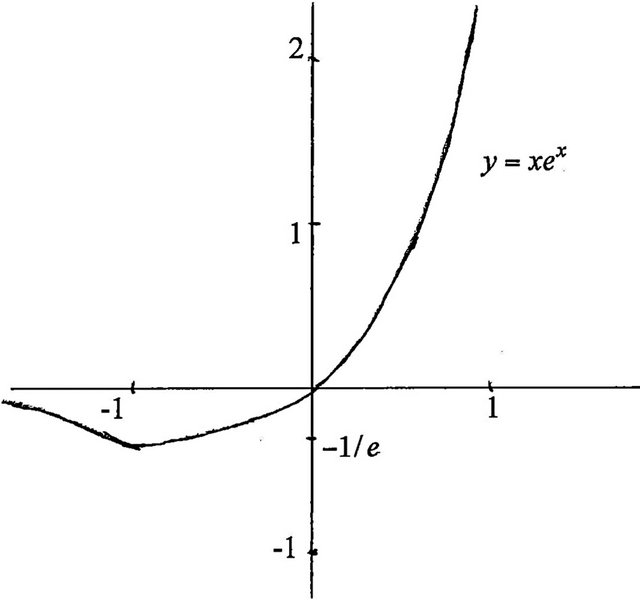
The exponential function  is defined for all real x, but has a codomain of
 . This function (Figure 1(a)) is the product of two elementary functions, each defined on the entire real line, and each being one-to-one; but the product is not injective. Consequently, if we restrict the domain to
 , then
  will possess an inverse, which is a function, and it’s this function that is now known as the (principal) Lambert W function (Figure 1(b)), written as
 . An alternative branch for W would be defined for that portion of
  when
when . We won’t consider that situation in this article.
Several function values of W are easy to computesuch as .
. and
and . The value of
 , known as the omega constant, has the approximate value 0.567143. The number
  is, in some sense, a distant cousin of the golden ratio
 , since
  is a solution to
 , and
, and  is the solution to
 , and
, and  is the linear Maclaurin approximation to
  (Figure 2). Since W is the inverse of
 , it follows that
 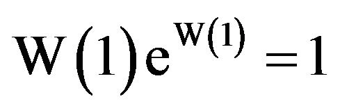 and that the slope of the curve in Figure 1(b) at the point
 is
is .
.
3. Computation
A natural question is how to compute arbitrary values of . One result, from the Lagrange inversion theorem, asserts that the Lambert W function has the Taylor series expansion [6,7]
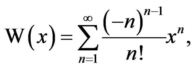 (1)
(1)
which, unfortunately, has a radius of convergence of merely . Since the denominator n! grows rapidly it’s
 (a)
(a)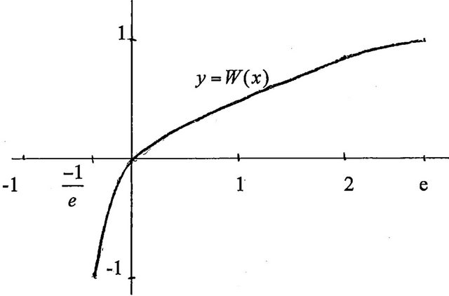 (b)
(b)
Figure 1. (a) Graph of ; (b) Graph of W(x),
 .
.
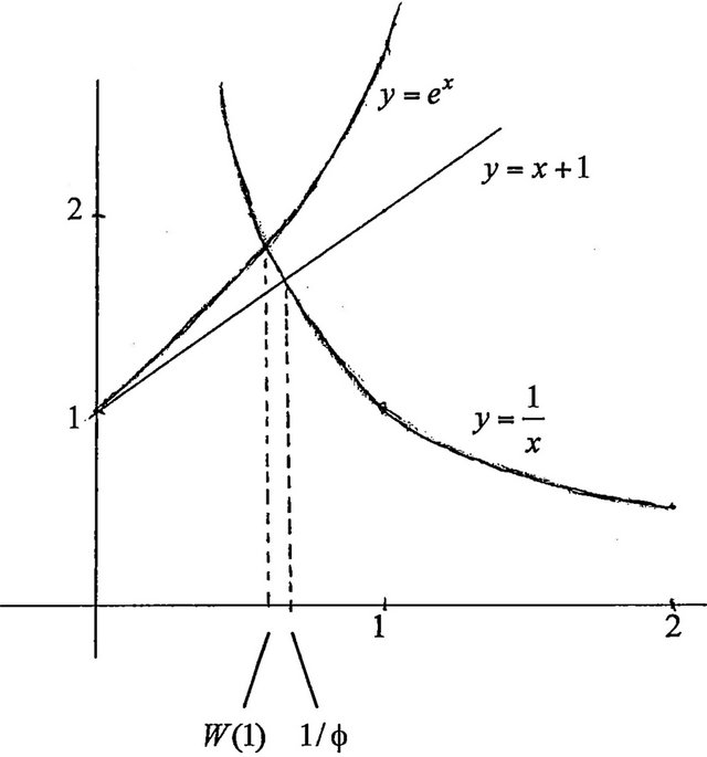
Figure 2.  and
and .
.
advantageous to write the series with the coefficients defined recursively as , with
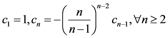 . This recursion lends itself to easy programming evaluation. Testing this, with say a series of 150 terms (which is plenty, considering that
 ), with
 , we obtain a partial sum value of
 , which differs from the exact value of
  by 0.0000003. We also note that
 , so the use of the series is justified.
On the other hand, a TI-graphing calculator returns “overflow error” if we try to determine , primarily since the coefficients grow rapidly.
Suppose that  and we wish to compute
 .
.
One possibility is the series
 (2)
(2)
where 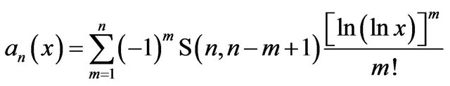 and
and
 denotes a Stirling number of the first kind [3]. The series (2) is somewhat impractical to use because of the difficulty in determining
 ; it turns out to be more useful to employ some standard numerical schemes for approximating
 .
.
First, setting , we need to solve
 . Defining the function g by
 , we use Newton’s method to approximate y in
 . This gives
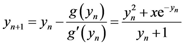 . To determine
 , for example, starting with an initial approximate of
 , after 7 more iterations we get
  , which is an excellent approximation to
  because
  returns 2 on the calculator. If x is a relatively small number, then an initial approximate of 0 will suffice for the algorithm; but if x is large, then ln x can be chosen for
 . For instance, if
 , choose
 , and after 5 iterations we get W(10) ≈ 1.745528003.
Newton’s method is a favorite iteration scheme for many because of its simplicity, though the convergence, quadratic in general, is typically relatively slow. A faster choice is furnished by Halley’s method (of Halley’s comet fame), which produces cubic convergence, and happens to be the choice implemented by the software Maple; this scheme gives [8]
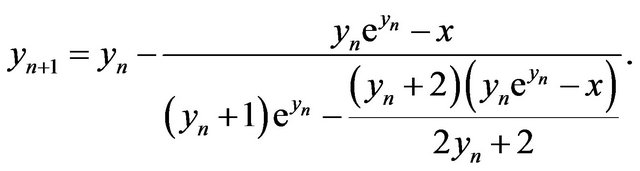
Employing this gives W(10) ≈ 1.745528003 after 3 iterations. This complex looking scheme is actually what you get when you apply Newton’s method to the function
 [9]. An alternative root-finding scheme, using continued fraction expansion, is described in [10].
4. Calculus
We know that since  is an increasing and differentiable function for all
  then its inverse
  is likewise increasing and differentiable for all
 .
.
Differentiating this latter equation with respect to y, we obtain
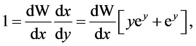
so
 (3)
(3)
In particular, 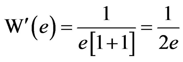 , and similarly,
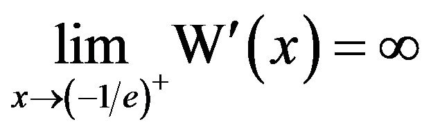 . What about
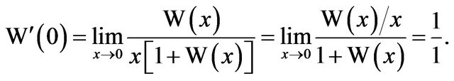
  the right-hand side of (3) is indeterminant at
 , but division of both sides of (1) by x and taking the limit as
  give
give
 . This yields
For large x, the graph of  bears strong resemblance to
 , since from (2) we have
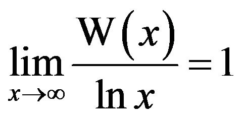 although we have to be careful here because the difference
  increases without bound as
 ![]() [7]. The graph of
[7]. The graph of , like that of
 , is concave downward for all x since
  is concave upward. If we differentiate (3), and omit the argument x for brevity, then
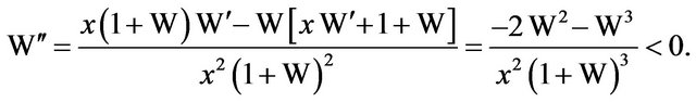
Rewriting  as
as 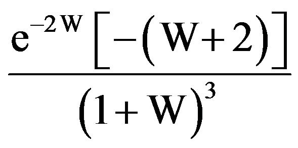 puts this into the form which fits the general case for
  [5]. In fact, from this form, we readily see that there is a point of inflection on the curve when
 , which actually falls on the other branch of the W function.
Continuing along the calculus vein, we should examine, if possible, the integral of . To this end, recall that
  iff
iff . Thus,
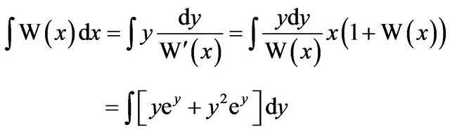
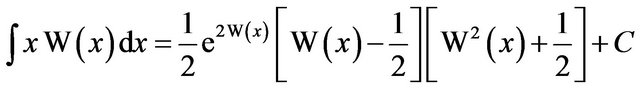
and integrating this last integral by parts, we obtain
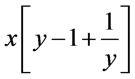 , which now gives
 (4)
(4)
In particular, the area of the region bounded by the curve , the x-axis, and the line
 ![]() is, therefore,
is, therefore,
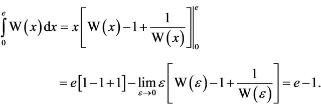
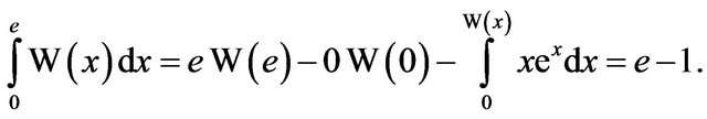
We note this result agrees with evaluating the integral via inverse functions [11], because then
Other integrals, involving functions containing W, can be computed, some just with a special change of variable [6]. For instance,
 .
.
The function  is concave up, connecting
and , hence its area
 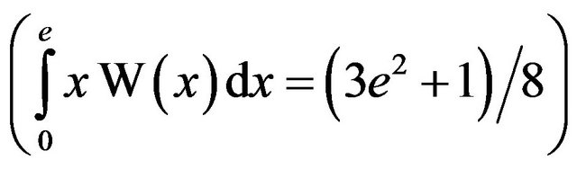 is less than
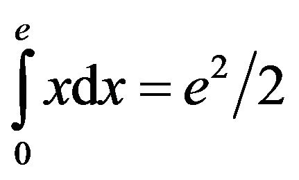 . Similarly we find
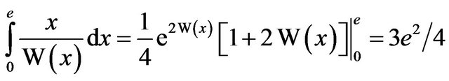 , and this is greater than
  since
since  is increasing and concave down from
 to
to .
.
5. Applications
An article appeared in the February, 2000, issue of FOCUS, the newsletter of the Mathematical Association of America, touting the merits of the W function as a candidate for a new elementary function to be studied in schools and to be included in textbooks [12]. The rationale for this was that not only is W a radically different function from the traditional elementary functions of polynomials, rationals, exponentials, logarithmics, and trigonometrics, but its calculus provides a wealth of interesting, and powerful, applications. A number of these are mentioned in a paper by Corless et al., where they describe such applications as enumeration of trees, combustion, enzyme kinetics, linear delay equations, population growth, spread of disease, and the analysis of algorithms [3]. An article [13] by Packel and Yuen shows that W is instrumental in determining the maximum range for a projectile with linear resistance (problems of this type have certainly been important for several thousand years). The solution for the current in a series diode/resistor circuit can also be written in terms of W. Applications of W are found in complex cases involving atomic, nuclear, and optical physics. The first physics problem to be solved explicitly in terms of W was one in which the exchange forces between two nuclei within the hydrogen molecular ion  were calculated [14]. Several other cases involve generalized Gaussian noise, solar winds, black holes, general relativity, quantum chromodynamics, fuel consumption, Stirling’s formula for n!, cardiorespiratory control, water-wave heights in oceanography, enumeration of trees in combinatorics, and statistical mechanics [5,15-17]. A really interesting analog of
  is given by Dan Kalman [18], where he defines a function glog, similar to W, in that glog is the inverse to
 . The glog function bears a strong resemblance to W, possessing similar properties and useful common applications, such as solving exponential-linear equations. The two functions are intimately related by
 and
and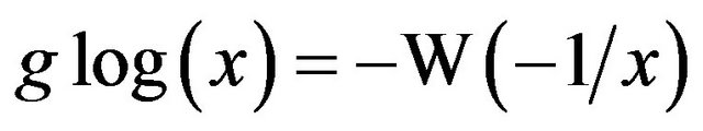 .
.
In the remainder of this article I wish to focus on a couple of applications dealing with ordinary algebraic equation solving.
6. Algebra
In a high-school precalculus course one might be presented with the elementary equation  to solve. Now, instead, let’s solve a similar equation
 , which means that it won’t suffice to begin by taking the logarithm of both sides. Instead, we proceed as follows:
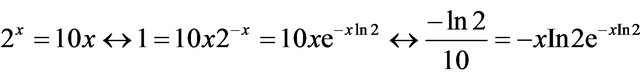
Since the right-hand side of this last equation is of the form , and since we know
  iff
iff then
then , or
, or .
.
Using Kalman’s glog function we can solve 
and get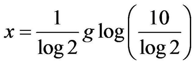 . Since
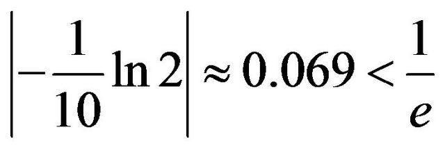 we can use (1) to approximate
 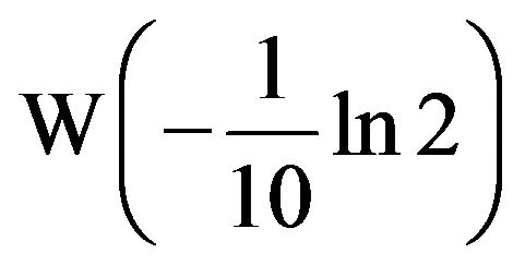 and get −0.0746900848, so x = 0.1077550149. Checking, we find 2x = 1.07755015 = 10x.
The equation  is a special case of a more general setting
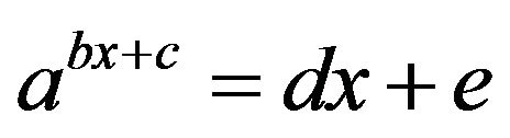 , where we assume the base
  and where neither b nor d equals zero. The substitution
 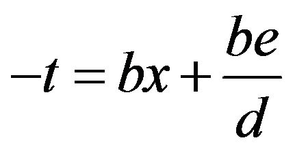 then gives
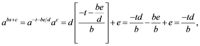
and, thus,
Multiplication of both sides by  gives
gives
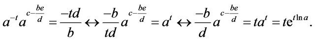
 , which now has the form
 , so
, so  or
or 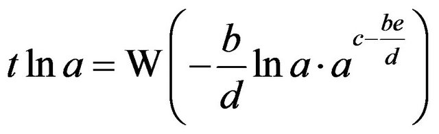
and, hence,
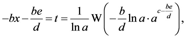
that is, 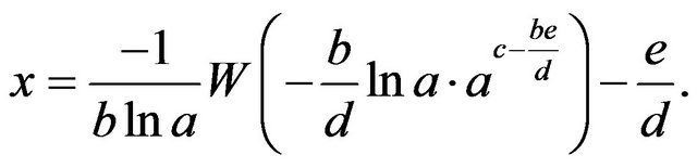
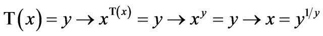
Another interesting algebraic application involves the infinite tower of exponents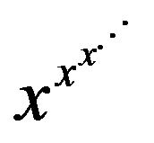 , which will be denoted by
 . To solve the particular equation
  one might argue that this is equivalent to
 , in which case we have
 , so
, so , which is the correct solution to
  But what about T(x) = 3, T(x) = 4, or T(x) = y. It stands to reason that as y increases, so does x. But with
 , we can write this as
 , or
, or , so
, so  again! Something isn’t right.
The problem lies with the domain of T. We find in [19] that the infinite tower of exponents is only defined (i.e.its interval of convergence) for , or approximately
 . So if x is selected from this interval, what is
 ? If we set
  then
then
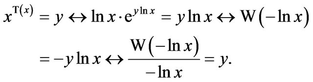 .
.
Note also that  when
when , and the above expression for y gives a function continuous at
 since
since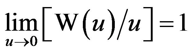 . Hence, if
 , then
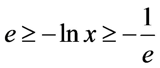 , so
, so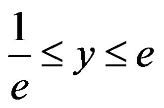 , and this is why the equation
  is solvable, but
  is not.
The graph of T is therefore an increasing function with domain  and range
 . It also passes through the two obvious points of
 and
and . What else can we deduce? Checking for differentiability, we have from (3),
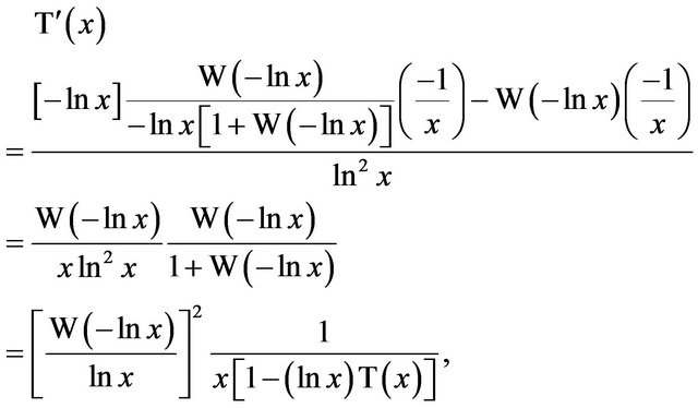
and since the limit of this expression is 1 as , then
 , and hence
  is never 0, so T is always strictly increasing. The following small table (Table 1) of values will prove helpful.
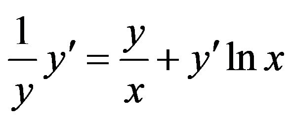
Alternatively, we could have found  by implicit differentiation of
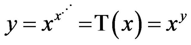 . Thus
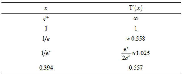
Table 1. Some derivative values.
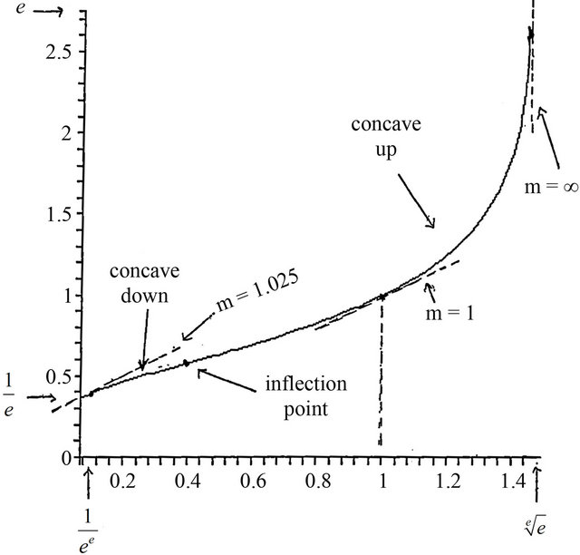
Figure 3. Graph of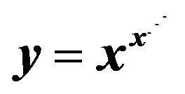 .
.
 or
or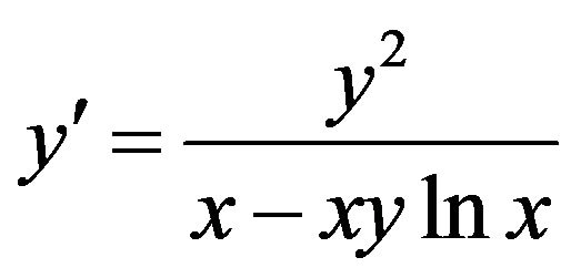 ; so again
 . Use of this form for easier access to
  then gives, after some algebraic manipulations and cancellations,
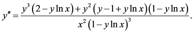
This complex expression appears to yield negative values for all  and positive values for all
 , and
, and . Hence, we have an inflection point at
 . Also
 . Putting all of these pieces of the puzzle together, we obtain a decent graph of T, as shown in Figure 3.
The tower function T must necessarily possess an inverse . We note then that
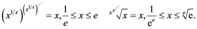
and, consequently, this inverse is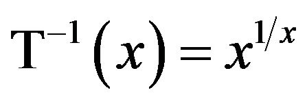 . Composition of the two functions give the interesting pair of identities,
REFERENCES
- J. J. Gray and L. Tiling, “Johann Heinrich Lambert, Mathematician and Scientist,” Historia Mathematica, Vol. 5, No. 7, 1978, pp. 13-14. doi:10.1016/0315-0860(78)90133-7
- B. Hays, “Why W,” American Scientist, Vol. 93, No. 2, 2005, pp. 104-108.
- R. M. Corless, G. H. Gonnet, D. E. Hare, D. J. Jeffrey and D. E. Knuth, “On the Lambert W Function,” Advances in Computational Mathematics, Vol. 5, No. 1, 1996, pp. 329-359.
- L. Euler, “De Formulis Exponentialibus Replicates,” Leonhardi Euleri Opera Omnia, Ser. 1, Opera Mathematics, Vol. 15, 1927, pp. 268-297.
- F. Chaspeau-Blondeau and A. Monir, “Numerical Evaluation of the Lambert W Function and Application to Generation of Generalized Gaussian Noise with Exponent ½,” IEEE Transactions on Signal Processing, Vol. 50, No. 1, 2002, pp. 2160-2165. doi:10.1109/TSP.2002.801912
- R. M. Corless, G. H. Gonnet, D. E. Hare and D. J. Jeffrey, “Lambert’s W Function in Maple,” The Maple Technical Newsletter, Vol. 9, 1993, pp. 12-22.
- F. Olver, D. Lozier, et al., “NIST Handbook of Mathematical Functions,” Cambridge University Press, Cambridge, 2010.
- W. Ledermann, “Handbook of Applicable Mathematics,” Vol. III, John Wiley & Sons, New York, 1981. pp. 151- 152.
- G. Alefeld, “On the Convergence of Halley’s Method,” The American Mathematical Monthly, Vol. 88, No. 7, 1981, pp. 530-536. doi:10.2307/2321760
- F. N. Fritsch, R. E. Shafer and W. P. Crowly, “Solution to the Transcendental Equation wew = x,” Communications of the ACM, Vol. 16, No. 2, 1973, pp. 123-124. doi:10.1145/361952.361970
- F. D. Parker, “Integrals of Inverse Functions,” The American Mathematical Monthly, Vol. 62, 1955, pp. 439-440. doi:10.2307/2307006
- F. Gouvea, Ed., “Time for a New Elementary Function?” FOCUS (Newsletter of Mathematics Association of America), Vol. 20, 2000, p. 2.
- E. W. Packel and D. S. Yuen, “Projectile Motion with Resistance and the Lambert W Function,” The College Mathematics Journal, Vol. 35, No. 5, 2004, pp. 337-350. doi:10.2307/4146843
- S. R. Valluri, D. J. Jeffrey and R. H. Corless, “Some Applications of the Lambert W Function to Physics,” Canadian Journal of Physics, Vol. 78, No. 9, 2000, pp. 823- 831.
- J. M. Borwein and R. M. Corless, “Emerging Tools for Experimental Mathematics,” The American Mathematical Monthly, Vol. 106, No. 10, 1999, pp. 889-909. doi:10.2307/2589743
- S. R. Cranmer, “New Views of the Solar Wind with the Lambert W Function,” American Journal of Physics, Vol. 72, No. 11, 2004, pp. 1397-1403. doi:10.1119/1.1775242
- D. P. Francis, K. Willson, L. C. Davies, A. J. Coats and M. Piepoli, “Quantitative General Theory for Periodic Breathing in Chronic Heart Failure and Its Clinical Implications,” Circulation, Vol. 102, No. 18, 2000, pp. 2214- 2221. doi:10.1161/01.CIR.102.18.2214
- D. Kalman, “A Generalized Logarithm for ExponentialLinear Equations,” The College Mathematics Journal, Vol. 32, No. 1, 2001, pp. 2-14. doi:10.2307/2687213
- R. Arthur Knoebel, “Exponentials Reiterated,” The American Mathematical Monthly, Vol. 88, No. 4, 1981, pp. 235-252. doi:10.2307/2320546