Applied Mathematics
Vol. 3 No. 3 (2012) , Article ID: 18093 , 8 pages DOI:10.4236/am.2012.33035
Temperature Distributions for Regional Hypothermia Based on Nonlinear Bioheat Equation of Pennes Type: Dermis and Subcutaneous Tissues
1Laboratoire d’Ingénierie des Microsystèmes Avancés, Département d’Informatique et d’Ingénierie, Université du Québec en Outaouais, Succursale Hull, Gatineau, Canada
2Department of Mathematics and Statistics, University of Ottawa, Ottawa, Canada
Email: *kengem01@uqo.ca
Received December 1, 2011; revised February 17, 2012; accepted February 27, 2012
Keywords: Regional Hypothermia; Dermis and Subcutaneous Tissues; Jacobi Elliptic Functions; Temperature-Dependent Blood Perfusion
ABSTRACT
We have used a nonlinear one-dimensional heat transfer model based on temperature-dependent blood perfusion to predict temperature distribution in dermis and subcutane-ous tissues subjected to point heating sources. By using Jacobi elliptic functions, we have first found the analytic solution corresponding to the steady-state temperature distribution in the tissue. With the obtained analytic steady-state temperature, the effects of the thermal conductivity, the blood perfusion, the metabolic heat generation, and the coefficient of heat transfer on the temperature distribution in living tissues are numerically analyzed. Our results show that the derived analytic steady-state temperature is useful to easily and accurately study the thermal behavior of the biological system, and can be extended to such applications as parameter measurement, temperature field reconstruct-ion and clinical treatment.
1. Introduction
The purpose of this work is to use Jacobian elliptic functions to construct a nonlinear heat transfer model in dermis and subcutaneous tissues. To predict the temperature in these two biological living tissues, we use a Pennes type of bio-heat transfer equation with a temperaturedependent blood perfusion term.
Since the pioneer work of Pennes [1] in which a linear mathematical model was proposed for describing the thermal interaction between human tissues and perfused blood, taking the effects of the metabolism into account, alternative nonlinear models for describing the heat exchange between tissues and blood have been developed [2-7]. The Pennes model assumes a constant rate blood perfusion within each type of tissues. However, it has been shown by several experiments and numerical simulations that physiological responses such as blood perfusion and metabolism in living tissues are temperaturedependent (see for example [5,8]). A more accurate description of the heat transfer in living biological tissues will then be obtained only by including, if possible, a temperature-dependent blood perfusion and a variable metabolic heat generation terms in Pennes equation.
By including a temperature-dependent blood perfusion term in Pennes equation, the temperature distribution in the living biological tissue at hand will be governed by a nonlinear time-dependent partial differential equation. In such biological tissues, the temperature will not be uniformly distributed in space and time. Moreover, it will be very difficult and even impossible to find analytical solutions of the governing equation; in such situations, only numerical solutions are attempted, and we talk of numerical temperature distribution in living biological tissues.
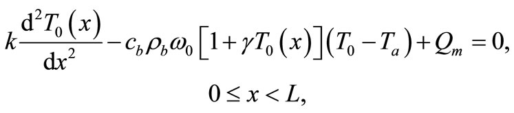
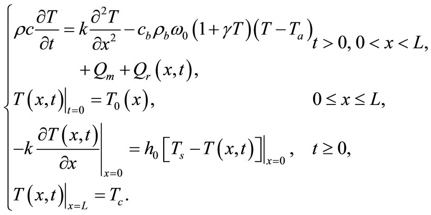
In the present work we use a Pennes type model of bio-heat transfer equation to numerically investigate temperature distribution in dermis and subcutaneous tissues; here, we include in Pennes equation a temperature-dependent blood perfusion term and maintain a constant metabolic heat generation term. Our investigation is based on the following one-dimensional (1D) modified Pennes bio-heat transfer model [8]:
 (1)
(1)
where ,
,  , k are the density, specific heat and thermal conductivity of the tissue, respectively,
  is the blood specific heat,
  is the blood density, T is the local tissue temperature,
  is the arterial blood temperature which is treated as constant,
  is time,
  is the metabolic heat production per volume, and
  is the heat deposited per volume due to spatially distributed heating (it is the external spatial heating),
  is the temperature-dependent blood perfusion, and
  denotes the distance from the skin surface to the body core. In this work, we take the temperature-dependent blood perfusion to be of the form [8]
 (2)
(2)
where  is the baseline perfusion and
  is the linear coefficient of temperature dependence. Because the interior tissue temperature usually tends to a constant a short distance from the skin surface, such as 0.02 - 0.03 m (see for example [9,10]), we consider in Equation (1) that
 , with
  m.
m.
The aim of this paper is to investigate via Equation (1) with blood perfusion (2) the temperature distribution in dermis and subcutaneous tissues in the hypothermia case when both skin surface and spatial heating are used. We restrict ourselves to positive temperatures. This paper is carried out in a case of hypothermia state where the tissue temperature is below 35˚C. In this work, we show how to increase the tissue temperature by applying point heating sources at different depths of the tissue and by controlling the equation parameters. The technique we used here is first to find the tissue temperature prior to heating, using Jacobi elliptic functions; this allows us to obtain the steady-state temperature (temperature of the tissue at time t = 0 s whose values are in the range of the temperature of a hypothermia of deep degree (below 20˚C). We then use the obtained steady-state temperature to numerically investigate the temperature distribution when the tissue is subjected to spatial point heating. The rest of the work is organized as follows: in Section 2 we use Jacobi elliptic functions to investigate the initial temperature distribution for the basal state of dermis and subcutaneous tissues. The numerical nonuniform (in time and space) temperature distribution is studied in Section 3, and our work is summarized in Section 4.
2. Investigation of the Initial Temperature Distribution for the Basal State of Dermis and Subcutaneous Tissues via Jacobi Elliptic Functions
Up to now, no author has applied Jacobi elliptic functions to analytically solve the steady-state problem of bioheat transfer equation with temperature-dependent blood perfusion. In most of the existing analytical studies, the solutions to the bioheat transfer problem for a steadystate are for temperature-independent blood perfusion, which may not be practical for real bio-thermal situations. Therefore it is still desirable to obtain possible way to analytically solve the most widely accepted Pennes’ equation in the bioheat field.
In this section, we investigate, by the means of Jacobi elliptic functions, the initial temperature field for the basal state of dermis and subcutaneous tissues. If we denote by  the steady-state temperature field prior to heating,
  the surrounding air temperature, and
  the apparent heat convection coefficient between the skin surface and the surrounding air under physiologically basal state (
 is also considered as an overall contribution from natural convection and radiation), then
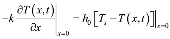
  will be the solution of the boundary value problem
 (3)
(3)
 (4)
(4)
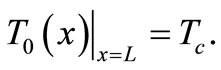
Because a biological body tends to keep its core temperature to remain stable, the body core temperature  is treated as a constant given by
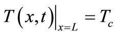 , whence the following additional boundary condition
 (5)
(5)
Because we work in a hypothermia case, the core temperature  will be chosen below 35˚C. If we multiply Equation (3) by
  and integrate the result, we obtain the first integral
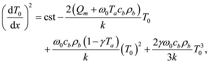 (6)
(6)
where cst in a constant of integration. Using the boundary condition (4), we find that
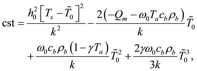 (7)
(7)
where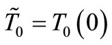 . The following notation,
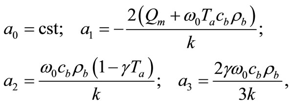 (8)
(8)
reduces Equation (6) to
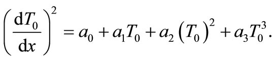 (9)
(9)
Particular solutions of Equation (9) can be found in terms of Jacobi elliptic functions [11]:
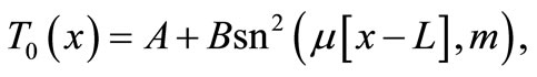 (10)
(10)
where 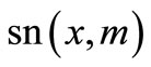 is the Jacobi elliptic sine function with modulus
  and A,
  ,
,  , and m are four constants verifying the nonlinear algebraic system
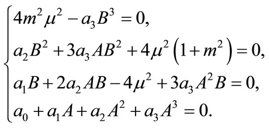 (11)
(11)
Because of our restriction on the positivity of  for all
 , we must have A > 0; moreover, if B < 0, the additional condition
 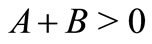 is required. Solving the first three equations of (11), we obtain, under the condition
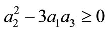 ,
,
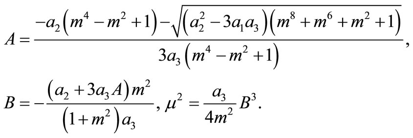 (12)
(12)
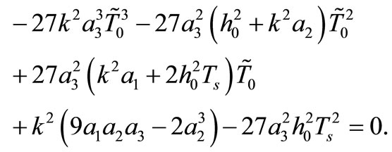
Inserting A in the fourth equation of system (11) yields
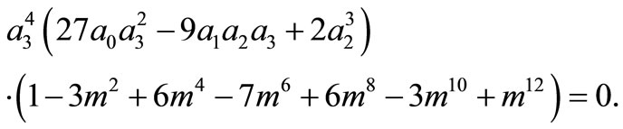
Because

for all m, we must have

Thus, the boundary value problems (3)-(5) will have solutions of the form (10) if and only if  and
and  The last condition means that the constant of integration, cst, in Equation (6) must satisfy the condition
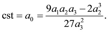 (13)
(13)
Comparing the right-hand sides of Equations (7) and (13) we obtain that the apparent heat convection coefficient  must satisfy the equation
 (14)
(14)
It follows from Equation (10) that 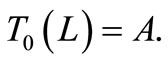 This last equality and condition (5) give
 , which together with the expression for A in Equation (12) give the equation
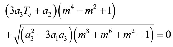 (15)
(15)
for determining m. A necessary condition for Equation (15) to have a solution is that 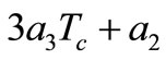 should be non-positive.
We summarize the obtained result as follows: if the initial temperature at skin surface satisfies Equation (14) and if  then the boundary value problems (3)-(5) admits particular solutions of the form (10) with
 , B, and
  given by Equation (12) and
  is a solution of Equation (15), where
 ,
,  , and
, and  are defined by Equation (8).
Solutions as (10) are expected to be very useful in a variety of bio-thermal practices: 1) for extreme situations where perfusion will change significantly with the external heating; 2) if the average perfusion in a specific temperature range was known (here, the analytical solution will provide intuitive temperature prediction); 3) for those bioheat transfers under small heating (in this case, a good accuracy from the analytical prediction can be expected).
Figure 1 shows the temperature distribution at the initial time t = 0 of dermis (left plot) and subcutaneous (right plot) tissues for different values of the linear coefficient γ of temperature dependence of blood perfusion. Here we have used for both dermis and subcutaneous tissues the following typical tissue parameters [12]: Ta = 37˚C, Ts = 15˚C, cb = 3500 J/kg˚C, Qm = 43800 w/m3, ω0 = 19 × 10–5 ml/100 g·min, ρb = 1060 kg/m3. As thermal conductivity of tissue, we used k = 0.45 w/m·˚C and k = 0.19 w/m·˚C for dermis and subcutaneous tissues, respectively. To investigate the effect of the linear coefficient of temperature dependenceγon the initial temperature distribution, we used three values of γ [13]: γ = 0.122, γ = 0.122597, and γ = 0.1226.
1) Dermis tissue: With the above equation parameters, we compute the elliptic moduli as m = 0.383359, m = 0.028886, and m = 0.0201884. Solution (10) then gives T0(0) = 12.7348˚C, T0(0) = 12.7˚C, and T0(0) = 12.6736˚C, respectively. Inserting these values of  in Equation (14) yields h0 = 35.142 w/m˚C, h0 = 35.0382 w/m2, and h0 = 34.7618 w/m2·˚C, respectively.
2) Subcutaneous tissue: For the subcutaneous tissue, we found m = 0.383359, m = 0.028886, m = 0.0201884 T0(0) = 12.7797˚C, T0(0) = 2.7043˚C, and T0(0) = 12.6927˚C; h0 = 44.0957 w/m2·˚C, h0 = 43.513 w/m2·˚C, and h0 = 43.328 w/m2·˚C.
The temperature curves of Figure 1 show that increased perfusion causes a decline in the local temperature, while the local temperature decreases with the elliptic modulus. Also, the temperature distribution becomes more oscillatory when the blood perfusion increases. Because dermis tissue and subcutaneous tissue differ only in thermal conductivity, we can also conclude from the plots of Figure 1 that an increased thermal conductivity causes a decline in local temperature.
3. Numerical Simulations
3.1. Numerical Techniques
Equation (1) with temperature-dependent blood perfusion (2) is a time-dependent nonlinear partial differential equation, and its numerical solutions can be obtained using a Crank-Nicolson scheme. In this section, we will stress on the solution of Equation (1) using a secondorder central difference scheme in space and a CrankNicholson type of scheme in time. The boundary conditions associated to Equation (1) is a segment that starts from the skin surface (x = 0) and ends at the body core (x = L) and is described as follows: a given temperature boundary condition is applied at the body core, i.e., T = Tc at x = L; a convective boundary condition is used at the skin surface, 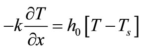 at x = 0, which is the normal case to which the skin surface is subjected. Because Equation (1) is time-dependent (first order differential equation in time), we need an initial condition. We will consider that prior to heating (i.e., at t = 0), the temperature at any depth x is
 , where
  is the steady-state temperature field found in the previous section (see Equation (10)); therefore
 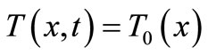 at t = 0. Mathematically, we will numerically solve the following initial boundary value-problem
 (16)
(16)
The Newton’s heating/cooling law
 means that, at any
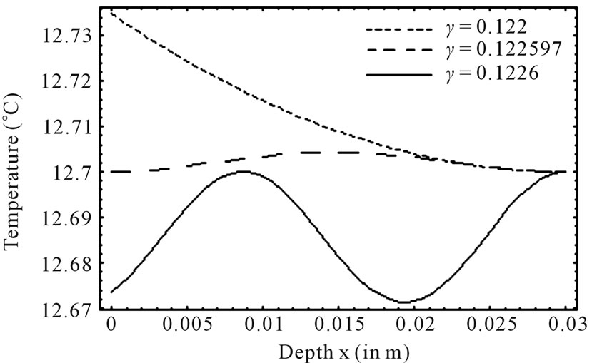
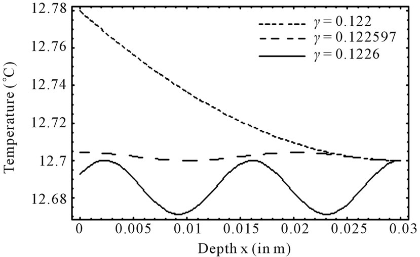
Figure 1. Effect of linear coefficient of temperature dependence γ of blood perfusion on initial temperature distribution in dermis (left plot) and subcutaneous (right plot) tissues in case of deep hypothermia (hypothermia of profound degree). As thermal conductivity, we used k = 0.45 w/m·˚C and k = 0.19 w/m·˚C for dermis and subcutaneous tissues, respectively.
time, the skin surface has exactly the same temperature as the heating/cooling medium: , where
  denotes the time-dependent temperature of the cooling medium. This condition is typical at the skin surface for thermal comfort analysis; it is also used for cancer hyperthermia.
Denote by  and h the time step discretization and the space mesh, respectively (here h is selected such that
  is a positive integer) and let
 ,
,  , and
, and ,
, . Let
. Let  be the scalar numerical value of the temperature at depth xj and time
 , i.e.,
  , and the vector value be
  an
an  matrix (column vector), where
 . Then, by applying a second-order central difference scheme in space and a Crank-Nicholson type scheme in time for solving problem (16), i.e., for finding all the
 , we find that the vector
  is the solution of an algebraic linear system of form
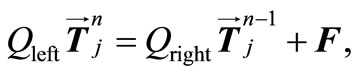 (17)
(17)
where  and
and  are two
  tridiagonal matrices and F an
  matrix (column vector); moreover
  is diagonally dominant. Hence, system (17) admits a unique solution
3.2. Numerical Experiments and Discussion
For the numerical simulation, we use the following parameters in Equation (1): Ta = 37˚C, Ts = 15˚C, Tc = 12.7˚C, cb = 3500 J/kg·˚C, Qm = 43800 w/m3, ω0 = 19 × 10–5 ml/100 g·min, ρb = 1060 kg/m3, ρ = 1200 kg/m3, c = 3300 J/kg·˚C. As thermal conductivity of the tissue, we used k = 0.45˚C and k = 0.19 w/m·˚C for dermis and subcutaneous tissue, respectively. The linear coefficient of temperature dependence γ is chosen among the following values: γ = 0.122, γ = 0.122597, and γ = 0.1226.  will be chosen in a way that Equation (10) will give a nontrivial solution
  of problems (3)-(5) (we point out that we shall use this solution as initial temperature distribution in the tissue). Although any spatial heating style like
  can be dealt with by the present numerical simulation, in this work we use only point heating to investigate the temperature response of the tissue [12,13]. Practical examples of point heating can be obtained in clinical treatments where heat is deposited by inserting a conducting heating probe in the deep tumor site or delivering thermal dose to it. Here, we use a point heating source of the form [12]
 (18)
(18)
where 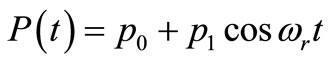 is the strength of the point heating source (it is the time-dependent heating power on the skin surface),
  is the Dirac delta function, and
  the location of the point heating;
  is a constant,
  the constant oscillation amplitude of sinusoidal heating,
  the heating frequency, and
  the scattering coefficient. The reason for choosing an oscillating heating, especially a sinusoidal heating, is that sinusoidal surface heating can be generated by an instrument with repeated irradiation from regulated laser and used to estimate the blood perfusion (see [14,15]). It follows from Equation (18) that
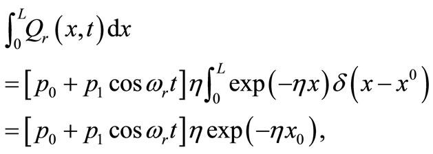
and this, of course, means that all the heat coming from the heating source is concentrated at the point  We will indicate for each example the values used for the heating parameters
 ,
,  ,
,  ,
,  , and
, and . In all the following examples, we have applied a point heating source at three different depths between the skin surface and the body core, exclusively; in fact, the skin surface is maintained at the same temperature as the cooling medium, and the body core temperature is maintained at
  (core temperature). Without loss of generality, we only work with dermis tissue, and all the obtained results may be transferred to subcutaneous tissue.
Figure 2 depicts the spatial and temporal temperature distributions of dermis tissue in the absence of spatial heating for γ = 0.1226. Due to the surface heating by the flowing of medium, the tissue temperature increases and is above the initial (steady-state) temperature. Because of the oscillatory aspect of the steady-state temperature field (see the plot of Figure 1 with γ = 0.1226), temporal temperature curves at the beginning of the process tend to be oscillatory (see the left plots on the top Figure 2). It is also important to point out that, at the beginning of the process (during about the first 110 s of the heating process), the temperature of the tissue at any depth is below the temperature at the skin surface (see left bottom plots). With time passing, the temperature first increases when one goes from skin surface to body core, reaches a highest value at some depth between x = 0.01285 m and x = 0.01585 m (see the bottom middle plots), and then decreases when one approaches the body core (see the right top plots). As one can see from the right plots (top and bottom), each point of the tissue reaches it stationary state after some duration of the process (near 3000 s). Moreover the highest temperature of each point during the process remains in the hypothermia range (see the top and bottom plots). Because of the continuous heating, the temperature of each point of the tissue increases rapidly in the early heating time and then slowly approaches its stationary value; this is easily seen from the bottom plots.
Figure 3 depicts spatial and temporal temperature distributions in dermis tissue in the presence of spatial heating when a point-heating source is applied. In this example, we used γ = 0.1226, p0 = 500,000/3 w/m2, p1 = 0 w/m2 and applied a point-heating source at three different points, namely, at x0 = 0.008571 m, x0 = 0.01585 m, and x = 0.02357 m. We first point out that all effects observed in the absence of spatial heating occur when a spatial heating source is applied; particularly, the temperature at each depth of the tissue increases gradually until it reaches steady-state. As the top plots show, the positions of higher temperatures stay at the site of the point sources. This is very beneficial, not only for hypothermia therapy, but also for hyperthermia therapy; in fact, one can selectively apply a point-heating source to heat the deep regional tumor in case of hyperthermia therapy. A comparison of Figures 2 and 3 show that the point-heating source may affect other points of the tissue only after a long heating time. A suitable localization of the heating source may prevent the destruction of the tissue cell that are outside the tumor region (in the case
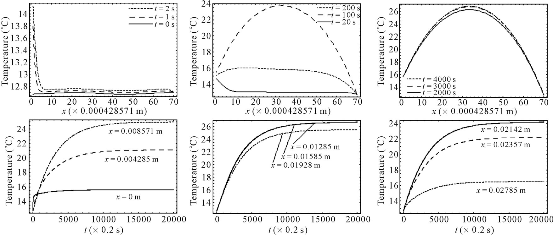
Figure 2. Spatial temperature distribution (top) and temporal temperature distribution (bottom) in dermis tissue (hypothermia of severe degrees) without spatial heating (Qr = 0). Here, we used γ = 0.1226, which corresponds to an oscillatory steadystate temperature field (see Figure 1).
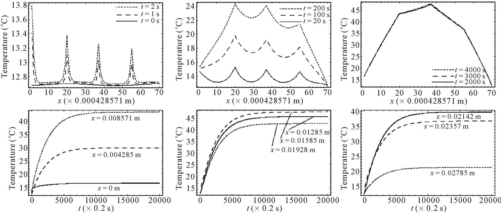
Figure 3. Spatial (top) and temporal (bottom) temperature distribution in dermis tissue subjected to a point-heating source applied at three different points: x0 = 0.008571 m, x0 = 0.01585 m, and x0 = 0.02357 m, with the heating parameters η = 20 m–1, p0 = 500,000/3 w/m2, and p1 = 0. For this figure, we have used γ = 0.1226, which corresponds to an oscillatory initial temperature (see Figure 1).
of hyperthermia therapy). In any case, the adoption of point-heating source is beneficial in medical therapy.
Figure 4 shows the spatial and the temporal temperature distributions in dermis tissues subjected to sinusoidal point-heating. Exactly as in the case of constant pointheating source, the local higher temperatures are in the position where the heating source is placed (see top plots). Also, the temperature of each point of the tissue increases gradually and after some time of heating, oscillates around a value that we may consider as its steady-state (see bottom plots). As we can see from the bottom plots, it is clear that there are about 12 cycles in the history of temperature variation, which is due to the value of the heating frequency . For
. For , the period
  of
of 
 is
is  seconds, and there are approximatively 12 cycles in 4000 seconds. Comparing the plots of Figures 3 and 4, we can conclude that one of the effects of sinusoidal heating is to increase the temperature in dermis tissue.
Figure 5 shows the temperature changes with time at the skin surface with and without spatial sinusoidal heating. In the case when point-heating source is applied, we
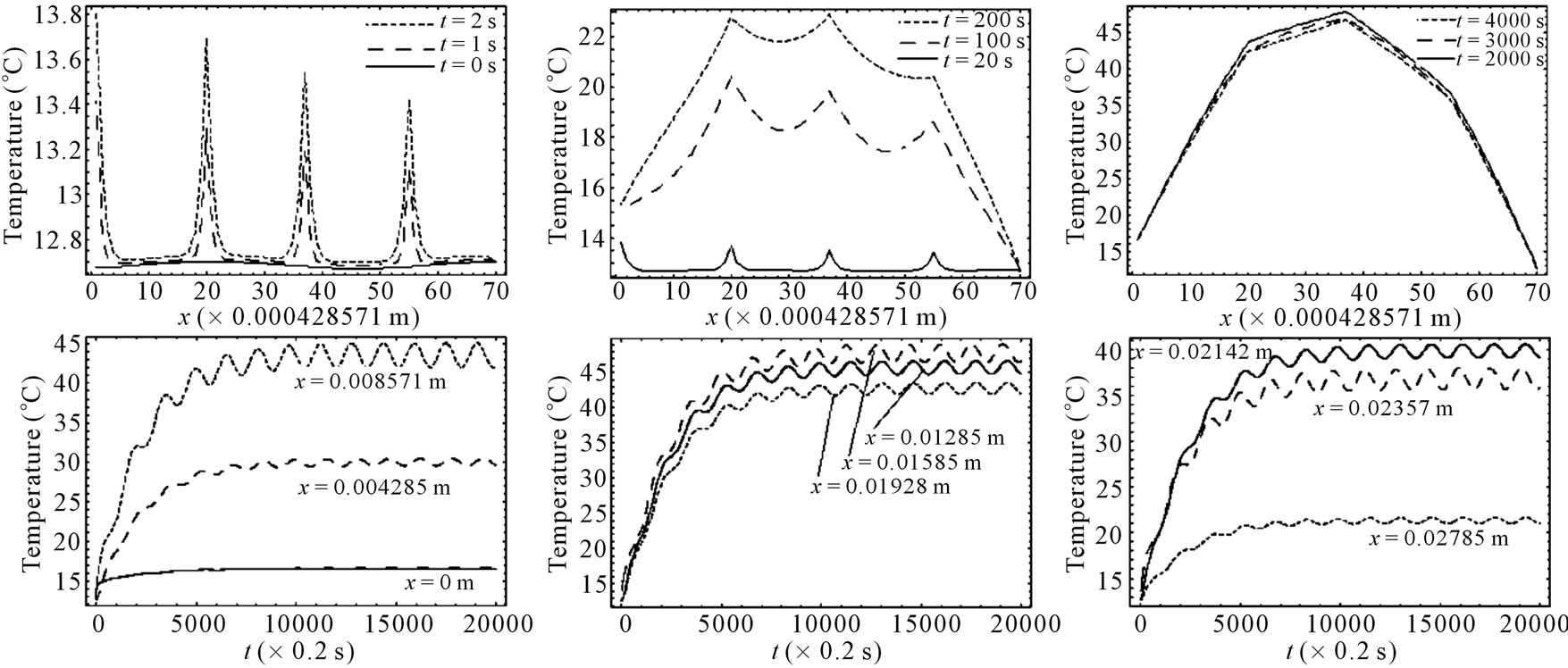
Figure 4. Spatial (top) and temporal (bottom) temperature distributions in dermis tissue subjected to a sinusoidal pointheating source applied at three different points: x0 = 0.008571 m, x0 = 0.01585 m, and x0 = 0.02357 m, with heating parameters η = 20 m–1, p0 = 500,000/3 w/m2, and m–1, p1 = 250,000/3 w/m2. For this figure, we have used γ = 0.1226, which corresponds to an oscillatory steady-state temperature field (see Figure 1).
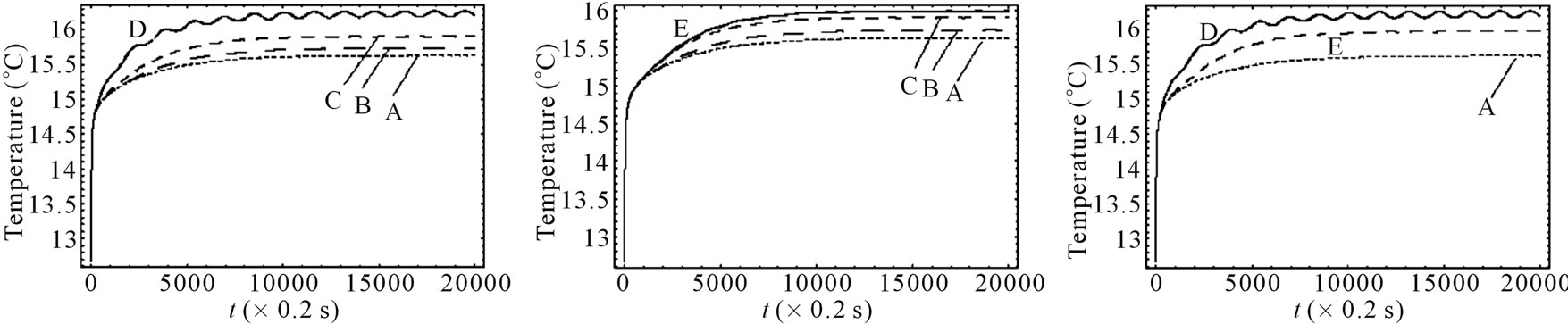
Figure 5. Effect of the position of a point-heating source on the temperature distribution at the skin surface. A: No spatial heating; B: One point-heating source placed at x0 = 0.02357 m; C: One point-heating source placed at x0 = 0.01585 m; D: One point-heating source placed at x0 = 0.008571 m; E: Two point-heating sources placed at x0 = 0.01585 m and x0 = 0.02357 m. The heating parameters were η = 20 m–1, p0 = 500,000/3 w/m2, and m–1, p1 = 250,000/3 w/m2. For this figure, we have used γ = 0.1226, which corresponds to an oscillatory initial temperature (see Figure 1).
distinguished first the situation when only a point-heating source is applied at a single point of the tissue and secondly, the situation when a point-heating source is applied at two points of the tissue. In the later case, a pointheating source is applied at two points of the tissue, far from the skin surface. This combination (a point-heating source applied at a single point, near and far from the skin surface, a point-heating source applied at two points far from skin surface) allows us to investigate how much a point-heating source may affect the temperature distribution at the skin surface which theoretically has the same temperature as that of heating/cooling medium. We found that the effect of a point-heating source on the temperature of the skin surface is negligible when the heating point is applied at a point far away from skin surface. Plots of Figure 5 allows us to conclude that the application of a point-heating source will increase the temperature of all points of the tissue and, consequentlyany two point-heating sources (point-heating source applied at two different points of the tissue) will interact between each other. It is seen from the right plots that the damage caused by one point-heating source placed near the skin surface may be more important than that caused by two point-heating sources placed far from skin surface.
4. Conclusions
The temperature distribution in dermis and subcutaneous tissues is numerically investigated in the hypothermia situation. The mathematical model we used is a timedependent bioheat equation of Pennes type containing a nonlinear term due to the blood perfusion term. In order to investigate the temperature distribution in the tissues in a hypothermia situation, we have used Jacobi elliptic functions to write out an analytical expression for the steady-state tissue temperature. Considering temperature to be time-dependent and considering the biological tissue to be subjected to a spatial point-heating source, the problem of temperature distribution in the tissue is solved by means of a second-order central difference scheme in space and a Crank-Nicholson type scheme in time.
We have conducted two numerical experiments, hypothermia and sinusoidal point-heating, which are typical heat transfer processes involved in soft tissues in biological bodies, such as heat therapy and skin burn. As results of our experiments, we found that: 1) the local highest temperature is where the heating source is placed; 2) the tissue in the heated position is more likely to be damaged (in the case of a higher strength of point heating source) than that in locations which are not heated; 3) the temperature of any point, near or far from the position of the heating source is affected by the heating source; 4) two heating sources will interact between each other.
In order to minimize the damage to the biological tissue due to the heating source, we recommend to consecutively place the point-heating source at the point of the tissue to be analyzed. We point out that the problem of sources isolation (how to place more than one pointheating source at different points of tissues such that two heating sources will not interact) remains unsolved, and we hope, in our future research, to bring out a positive result in this direction.
REFERENCES
- H. H. Pennes, “Analysis of Tissue and Arterial Blood Temperatures in the Resting Forearm,” Journal of Applied Physiology, Vol. 1, No. 2, 1948, pp. 93-122.
- A. Szasz and G. Vincze, “Dose Concept of Oncological Hyperthermia: Heat-Equation Considering the Cell Destruction,” Journal of Cancer Research and Therapeutics, Vol. 2, No. 4, 2006, pp. 171-181. doi:10.4103/0973-1482.29827
- C. K. Charney, “Mathematical Models of Bioheat Transfer,” Advanced Heat Transfer, Vol. 22, 1992, pp. 19-155. doi:10.1016/S0065-2717(08)70344-7
- P. Deuflhard and R. Hochmuth, “Multiscale Analysis of Thermoregulation in the Human Microvascular System,” Mathematical Methods in the Applied Sciences, Vol. 27, No. 8, 2004, pp. 971-989. doi:10.1002/mma.499
- T. R. Gowrishankar, D. A. Stewart, G. T. Martin and J. C. Weaver, “Transport Lattice Models of Heat Transport in Skin with Spatially Heterogeneous, Temperature-Dependent Perfusion,” BioMedical Engineering on Line, Vol. 3, No. 4, 2004, pp. 1-17.
- A. Lakhssassi, E. Kengne and H. Semmaoui, “Modified Pennes’ Equation Modelling Bio-Heat Transfer in Living Tissues: Analytical and Numerical Analysis,” Natural Science, Vol. 2, No. 12, 2010, pp. 1375-1385. doi:10.4236/ns.2010.212168
- C. R. Davies, G. M. Saidel and H. Harasaki, “Sensitivity Analysis of One-Dimensional Heat Transfer in Tissue with Temperature-Dependent Perfusion,” Journal of Biomechanical Engineering, Vol. 119, No. 1, 1997, pp. 77-80. doi:10.1115/1.2796068
- J. Lang, B. Erdmann and M. Seebass, “Impact of Nonlinear Heat Transfer on Temperature Control in Regional Hyperthermia,” IEEE Transactions on Biomedical Engineering, Vol. 46, No. 9, 1999, pp. 1129-1138. doi:10.1109/10.784145
- J. Liu and L. X. Xu, “Estimation of Blood Perfusion Using Phase Shift in Temperature Response to Sinusoidal Heating at the Skin Surface,” IEEE Transactions on Biomedical Engineering, Vol. 46, No. 9, 1999, pp. 1037- 1043. doi:10.1109/10.784134
- S. Weinbaum, L. M. Jiji and D. E. Lemons, “Theory and Experiment for the Effect of Vascular Microstructure on Surface Tissue Heat Transfer—Part I: Anatomical Foundation and Model Conceptualization,” Journal of Biomechanical Engineering, Vol. 106, No. 4, 1984, pp. 321- 330. doi:10.1115/1.3138501
- P. F. Byrd and M. D. Friedman, “Handbook of Elliptic Integrals for Engineers and Scientists,” 2nd Edition, Springer-Verlag, Berlin, 1971.
- Z. S. Deng and J. Liu, “Analytical Study on Bioheat Transfer Problems with Spatial or Transient Heating on Skin Surface or Inside Biological Bodies,” Journal of Biomechanical Engineering, Vol. 124, No. 6, 2002, pp. 638-650. doi:10.1115/1.1516810
- S. Karaa, J. Zhang and F. Yang, “A Numerical Study of a 3D Bioheat Transfer Problem with Different Spatial Heating,” Mathematics and Computers in Simulation, Vol. 68, No. 4, 2005, pp. 375-388. doi:10.1016/j.matcom.2005.02.032
- W. Shen and J. Zhang, “Modeling and Numerical Simulation of Bioheat Transfer and Biomechanics in Soft Tissue,” Mathematical and Computer Modelling, Vol. 41, No. 11-12, 2005, pp. 1251-1265. doi:10.1016/j.mcm.2004.09.006
- A. T. Patera, B. B. Mikic, G. Eden and H. F. Bowman, “Prediction of Tissue Perfusion from Measurement of the Phase Shift between Heat Flux and Temperature,” Proceedings of ASME Winter Annual Meeting, Advances in Bioengineering, 1979, pp. 187-191.
NOTES
*Corresponding author: kengem01@uqo.ca, ekengne@uottawa.ca.