Modern Economy
Vol.5 No.1(2014), Article ID:42133,17 pages DOI:10.4236/me.2014.51005
Revisiting the J-Curve for Japan
1Faculty of Economics, Seikei University, Musashino-shi, Japan
2School of International Liberal Studies, Waseda University, Tokyo, Japan
Email: *mono@econ.seikei.ac.jp, baak@waseda.jp
Copyright © 2014 Masanori Ono, SaangJoon Baak. This is an open access article distributed under the Creative Commons Attribution License, which permits unrestricted use, distribution, and reproduction in any medium, provided the original work is properly cited. In accordance of the Creative Commons Attribution License all Copyrights © 2014 are reserved for SCIRP and the owner of the intellectual property Masanori Ono, SaangJoon Baak. All Copyright © 2014 are guarded by law and by SCIRP as a guardian.
Received November 9, 2013; revised December 9, 2013; accepted December 16, 2013
KEYWORDS
J-Curve; S-Curve; Structural Change
ABSTRACT
This paper investigates Japanese trade to see whether the J/S-curve phenomenon between net exports and the terms of trade is observed in the data from 1980Q1 to 2008Q3. Based on the results of a VAR stability test, the aggregate trade data are endogenously split into three sub-period data sets, with the J/S-curve present in the last two. The J/S-curve may stem from the increasing share of China and the oil-exporting countries in Japanese trade. In fact, the J/S-curve is observed in the bilateral trade data with those countries but not in the data with Korea or the United States.
1. Introduction
1.1. Background Information
For the last few decades, as the Japanese economy has suffered from a stagnant or recessive domestic market, Japan has actively sought out foreign markets to compensate for sluggish domestic demand, resulting in an increase in the ratio of trade volume to GDP. The exportto-GDP ratio and the import-to-GDP ratio rose to 17.7% and 17.5%, respectively, in 2007; they then declined to 15.2% and 16.1%, respectively, in 2011. But the ratios are far higher than their values in the 1990s. For example, the highest export-to-GDP ratio in the 1990s was 10.8% in 1998, and the highest import-to-GDP ratio in the same decade was 9.7% in 1997. In addition, the quarterly trade balance had always been positive for the last two decades until 2008Q31.
Since the subprime mortgage crisis, which began in the United States in 2008, world trade volume has decreased due to the global recession. Adding to the reduced external demand, the exporting companies of Japan suffered from the appreciating yen. The monthly exchange rate (period average) of the Japanese yen against the US dollar had been between 103.8 and 133.5 from 2000 to 2007. In the last three months of 2007, it was between 112.2 and 115.7, but it dipped below 100 in November of 2008 and dropped further, below 90, in November 2009. While the Japanese yen was appreciating, the trade balance of Japan sharply declined and became negative in the third quarter of 2008 for the first time since the first quarter of 1982. Even though the trade balance of Japan recovered to a positive value in the second quarter of 2009, it became negative again in the second quarter of 2011 as the value of the yen further appreciated, and since then Japan’s trade balance has been negative despite recent depreciation of the yen.
In general, to understand an open economy, it is essential to understand the dynamics of trade balance, exchange rates, and the relationship between those two variables. This is particularly important if external demand forms a substantial share of total demand and the currency value is quite volatile.
With this background, this paper sets out to investigate how the Japanese trade balance is related to changes in terms of trade and real exchange rates. In particular, this paper aims to detect the presence of Jand S-curves in the Japanese economy over the past three decades and to explore whether there have been structural breaks in the curves.
Since its introduction by [1], the J-curve phenomenon, caused by slow volume adjustments to a change in the exchange rate, has been frequently reported by many researchers (see [2]). A country’s trade balance deteriorates just after the devaluation in the currency, but it gradually improves due to an increase in the volume of exports and a decrease in the volume of imports. Therefore, the Jcurve emerges from the relationship between trade balance and time. When the currency appreciates, the same reasoning leads to an inverted J-curve.
In addition, [3] simulates an open macroeconomic model with a time-to-build structure in capital formation. The simulation and empirical investigation for major industrial countries produce an S-curve in the cross-correlations between the trade balance and an exchange rate. In fact, the right-hand side of the S-curve (that is, the causality from lagged exchange rates to trade balance) accords with the J-curve phenomenon. In the meantime, the left-hand side of the S-curve (the one from lagged trade balance to exchange rates) indicates exchange rate adjustments to trade imbalances.
1.2. Literature Review
As the survey paper of [2] shows, a substantial amount of literature investigated the relationship between Japan’s trade balance and its exchange rate in the 1980s and 1990s. The exchange rate of the yen against the US dollar appreciated by 68% from 1985Q1 to 1987Q1, and by 19% from 1987Q1 to 1989Q2. Then the rapid appreciation drew many researchers’ attention to the J-curve phenomenon. For example, [4] estimated the magnitude of the J-curve during the period from 1985 to 1986. [5] simulated the J-curve shape during the period from 1985 to 1987. In contrast, the yen-dollar exchange rate depreciated by about 30% from 1995Q2 to 1997Q3. [6] then examined how the J-curve emerged from the depreciation4. [10] discovered some supportive evidence of a Jcurve in the bilateral trade data between Japan and two of its trading partners.
In this paper, we will revisit the J-curve phenomenon, taking into account the effect of changes in the international economic environment on the Japanese economy. Despite an extensive body of literature discussing the Jcurve issue with regard to Japan in the 1980s and 1990s, only a small number of papers have explored the same issue in the 2000s. Among them, [11] uses the data from 1973 to 2005 to analyze a J-curve and an S-curve, respectively, not only in the total trade of Japan but also in bilateral trade with major trading partners. They report the presence of an S-curve in Japan’s bilateral trade data with many of its trading partners. Using the data from 1980 to 2001, however, [12] reports the presence of the conventional J-curve phenomenon in Japan’s aggregate trade data but no evidence for the J-curve in the bilateral trade.
In the several months following November 2012, the value of the yen against the US dollar depreciated by about 25%, mainly due to the Abe administration’s economic policies (so-called Abenomics)5. [13, Chart 7] shows the J-curve effect with their economic model simulation, in which the depreciation of the yen since November 2012 first widens the trade deficit and then works to narrow it after January-March 2014.
To our knowledge, however, no recent paper has considered the possibility of a structural break6 due to drastic changes in the recent international trade environment surrounding the Japanese economy; therefore our understanding of the relationship between trade and exchange rates in Japan is still quite limited.
Employing a methodology similar to that of [11,14], this paper also examines both aggregate and bilateral trade data. However, it tries to further contribute to our understanding of Japan’s J/S-curve by considering the possibility of a structural break in the dynamics of Japan’s trade pattern and by focusing on more recent data. As is well known, the emergence of China in the world market has influenced many Asian countries, including Japan, and drastically changed the trade environment surrounding Japan.
For example, Figure 1 depicts Japanese international trade with its major partners. The most prominent change is a rapid increase in trade with China, which accelerated around 2002 and surpassed its trade with the United States in 2006. In addition, as oil prices increased, trade with oil-exporting countries surpassed trade with the euro area. If a J/S-curve phenomenon is observed in the bilateral trade with some trading partners but not in the trade with others, as reported by [10,12], then this may mean that Japan has experienced a structural break in the relationship between total trade balance and exchange rates over the decades as the share of each trading partner in the total trade of Japan has changed. Also, we look for a possible structural break in each bilateral trade.
2. Analysis of the Aggregate Trade Data
This section examines the S-curve dynamics in Japan’s
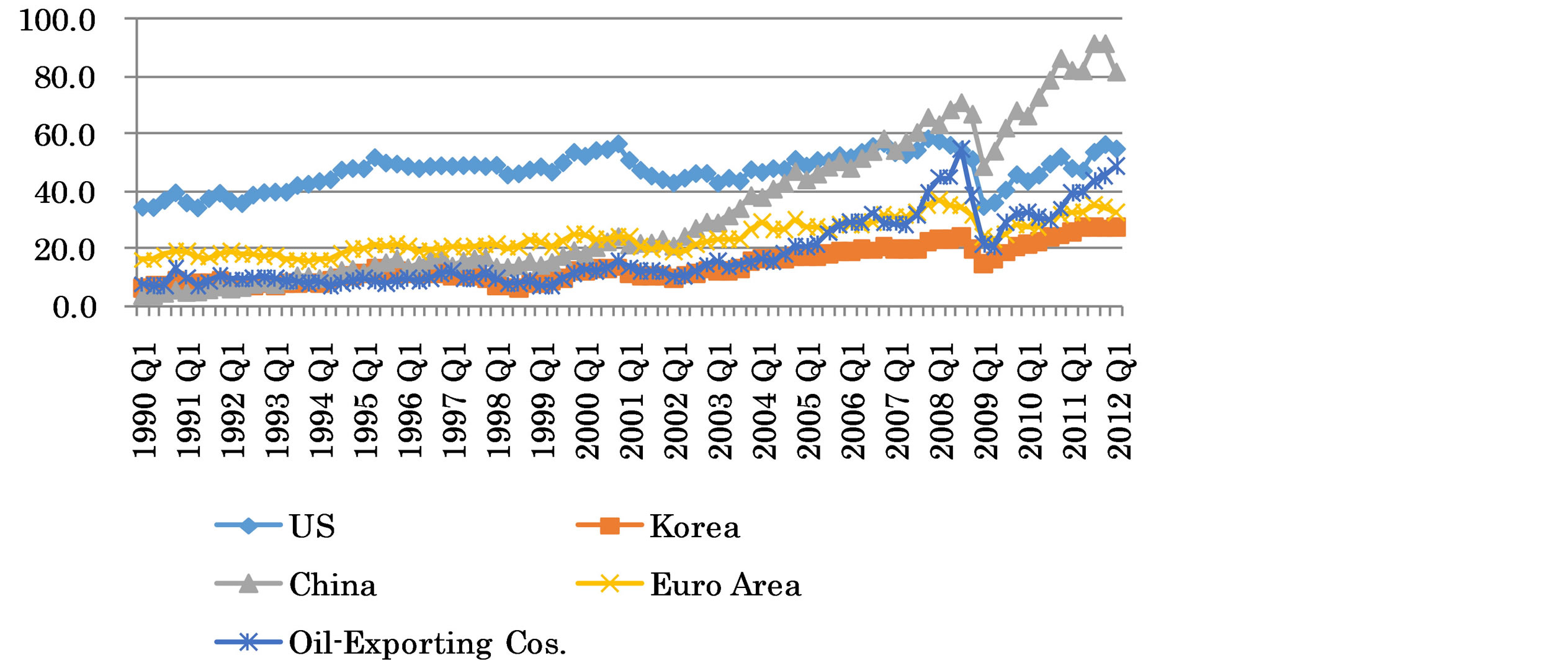
Figure 1. Trade of Japan with its major trading partners (US$ billion). Source: DOTS (IMF).
aggregate trade balance. We follow [11] to investigate the S-curve shape in the trade dynamics with exchange rates, and we extend our inquiry to test whether the Scurve shape has changed over the last few decades.
2.1. Data
Our sample period starts in 1980Q1 and ends in 2012Q4. However, we have excluded the data from 2008Q4 to 2012Q4 from our analysis because the VAR estimations indicated high instability after 2008Q37. Following [11], we define net exports (NX) as the ratio of net exports divided by GDP, and terms of trade (TOT) as the price of imports relative to the price of exports. We collected data for exports and imports from the Direction of Trade Statistics (DOTS) and those for prices and exchange rates from the International Financial Statistics (IFS). Both data sets are compiled by the IMF. For Japan’s GDP, we use the information released by Japan’s Cabinet Office. Table 1 depicts the variables and data source that we use in this section.
To obtain seasonally adjusted and detrended data, we have executed the following steps.
For NX (=net export /GDP):
1. Convert seasonally adjusted GDP data in Japanese yen into U.S. dollars by multiplying the GDP data by quarterly average exchange rates of the yen against the U.S. dollar.
2. Make a ratio of net exports in the U.S. dollar relative to the GDP obtained in Step 1. Note that the net exports figure (= exports – imports) obtained from IMF's DOTS is not seasonally adjusted.
3. Remove seasonality from the ratio derived in Step 2, using EViews’X-12 seasonal adjustment. We use the X-12 method with an additive component option because
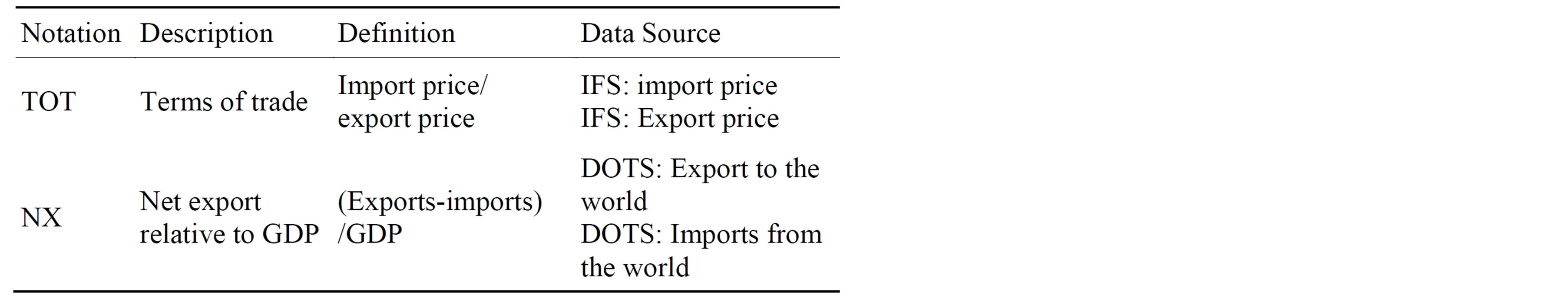
Table 1. Notation and the data source.
a multiplicative option in X-12 fails due to negative signs of net exports in some quarters.
4. Apply the Hodrick-Prescott filter (Lambda = 1600) to divide the series into trend and cycle parts.
5. The cycle part, which is equivalent to TB in the computation of the cross-correlation coefficient (COR) in [11, p. 488], is used as net exports (NX) in the J/S-curve analysis in this paper.
For TOT:
Apply the preceding Steps 3 to 4 to the ratio of the import price index relative to the export price index. The cycle part, which is equivalent to RE in COR in [11, p. 488], is used as the terms of trade (TOT).
Because structural breaks in the dynamics of a variable may conceal the presence of a unit root ([15]), in order to detect a unit root in NX and TOT we employ the S-L unit root test ([16]), which is robust in the presence of a structural break. As reported in Table 2, the null hypothesis of a unit root is rejected at the 5% significance level for all the variables tested.
2.2. J/S-Curve for the Full Sample Period (1980Q1-2008Q3)
In this section, we examine the S-curve shapes between TOT and NX in the full sample period (1980Q1-2008Q3) by using cross-correlations, impulse response functions, and Granger causalities.
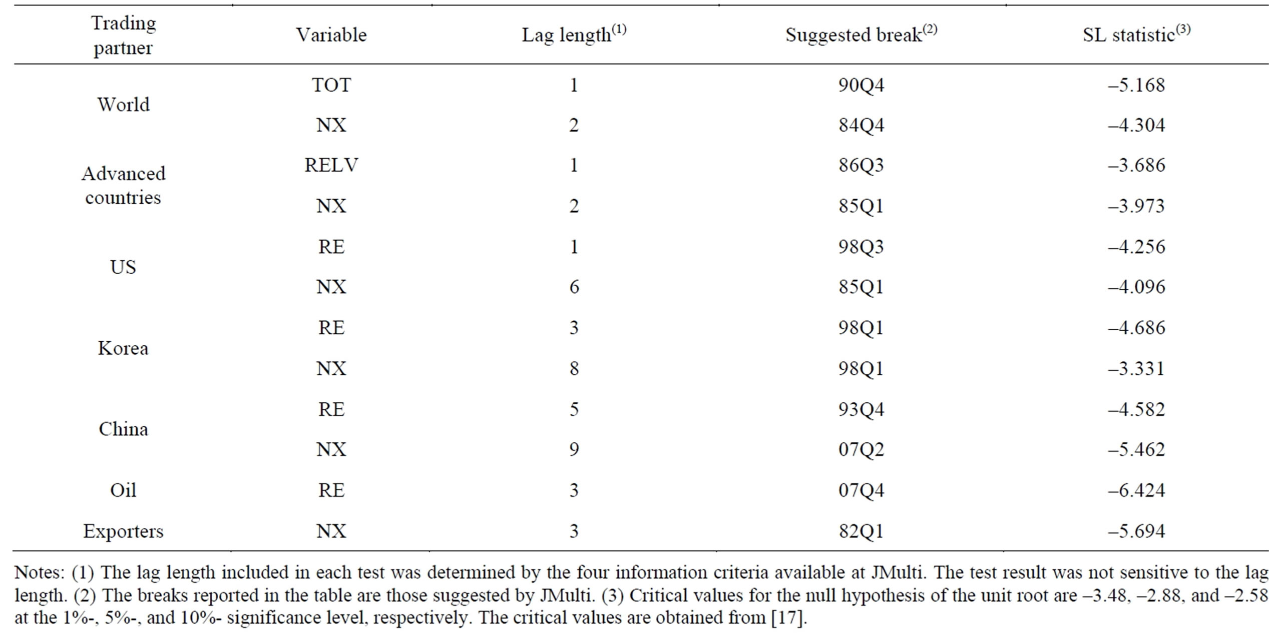
Table 2. SL unit root test with a structural break.
2.2.1. Cross-Correlations
First, we follow [11] to examine whether the S-curve shape appears in the cross-correlations between net exports and the terms of trade in the full sample period (1980Q3-2008Q3). Figure 2 illustrates the cross-correlations along with plus and minus twofold standard errors to show a statistical significance from zero. The J-shaped curve emerges from time 0, and the cross-correlation appears well below the minus twofold standard errors. On the other hand, the correlation goes above the plus twofold standard errors from times 4 to 14.
2.2.2. Impulse Response Functions
We continue our investigation of the S-curve using the VAR approach. For the VAR model, we use NXt and TOTt to form a vector of two variables; namely, Xt = (NXt, TOTt)’. To capture contemporaneous relations between shocks, we use the generalized impulse response function, which does not require orthogonalization of shocks8. Figure 3 illustrates the impulse response functions for the entire time period.
In the figure, we examine whether a response of NX to a shock in the TOT demonstrates the J-curve (that is, the right-hand side of the S-curve). The J-curve appears in the figure for a response of NX to a shock in the TOT. In addition, we also investigate whether a response of TOT to a shock in the NX exhibits the left-hand side of the S-curve. In the figure, the left-hand side of the S-curve also appears in reverse from side to side in the figure for a response of TOT to a shock in NX.
2.2.3. Granger Causalities
Using the preceding estimations of the VAR model, we evaluate how significantly TOT Granger-causes NX and vice versa. Table 3 reports the results. We reject the null hypothesis that TOT does not Granger-cause NX at the 1% significance level. On the other hand, we accept the null hypothesis that NX does not Granger-cause TOT at the 10% level. The causality from TOT to NX appears to be much stronger than the opposite influence.
2.3. Endogenously Determined Sample Periods
To reveal a structural break in the J/S-curve, we use the stability test for the VAR model, which was adopted by [19-22] among others. A structural break at one point in time in the VAR model indicates a structural change in the impulse response functions. Eventually, the J/S-curve projected in the impulse response functions changes its shape at that point. Hence this test can virtually reveal when a change in the J/S-curve takes place. Then the data are split into sub-periods, and we examine the S-curve shapes for each sub-period in the same way as adopted in the analysis of the aggregate data.
As an alternative to the VAR’s stability test, we may be able to test for equality in cross-correlations between TOT, NX(i) at each lead/lag i between two specific sample periods9. However, such a test stands on each i alone, not on all i’s. Therefore the equality test does not allow us to examine a change in the J/S-curve as systematically as does the VAR stability test.
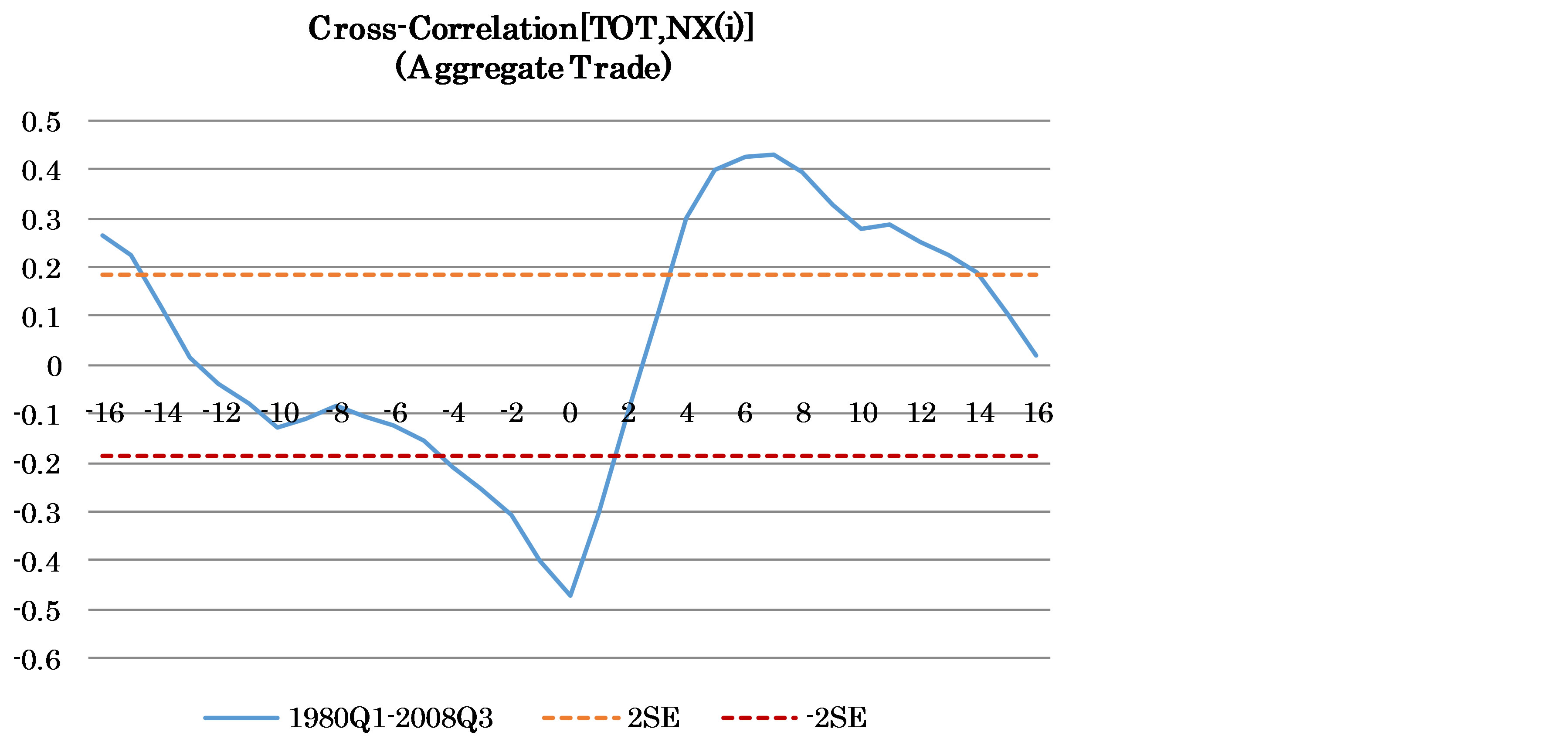
Figure 2. Cross-correlations.
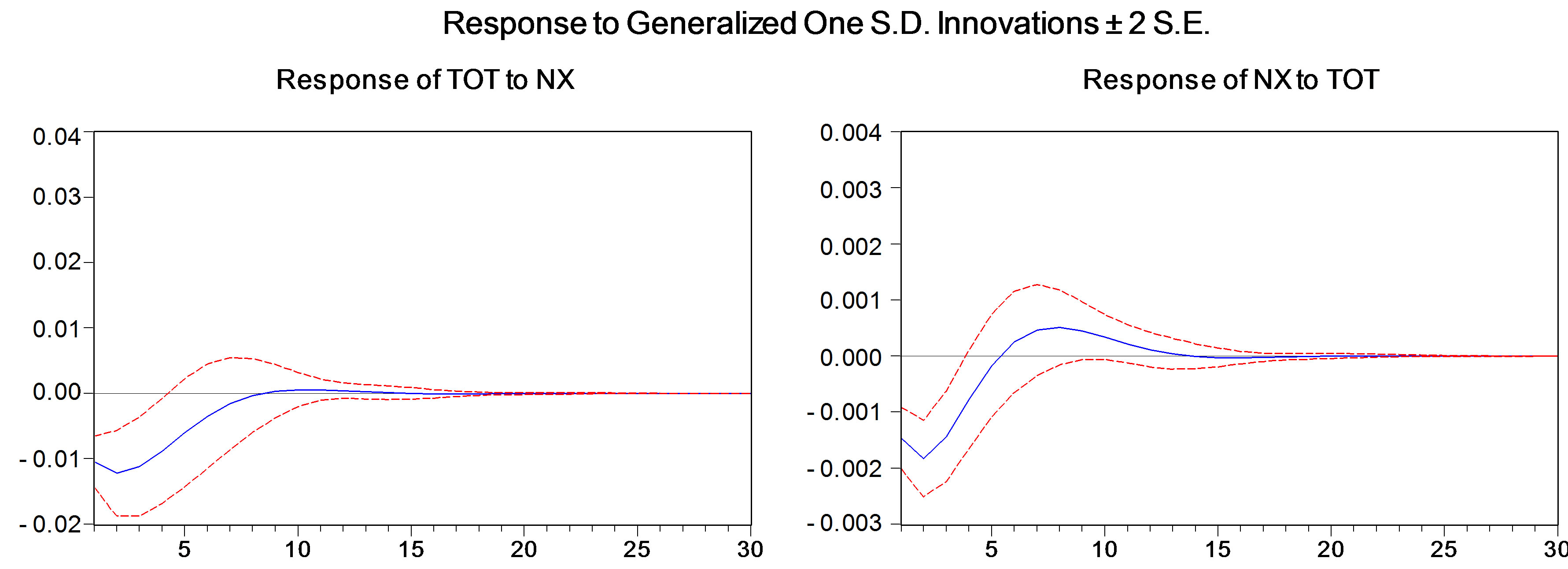
Figure 3. 1980Q1-2008Q3 (SIC: 2 lags).
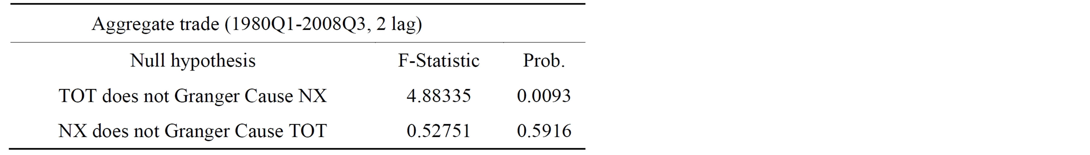
Table 3. Granger causality tests for the full sample period (1980Q1-2008Q3).
Specifically, the stability test employed in this paper is used to test for the following null hypothesis, H0:
 (1)
(1)
 for the first period (1 ≤ t ≤ i−1),
 for the second period (i ≤ t ≤ T).
H0:  and
and where
where ,
,
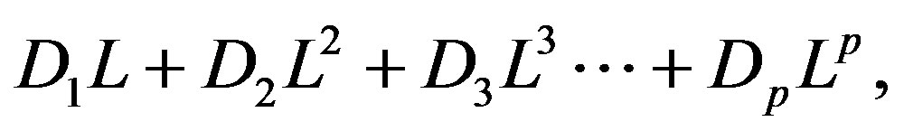 A0, A1, …Ap, D0, D1, … Dp are matrices of coefficients to be estimated, ηt is a vector of innovations, di is a vector of dummy variables, and T is an ending observation of the sample period. The null hypothesis for the stability test, H0, is that no structural change occurred between time i−1 and time i.
If we reject the null hypothesis at time i, we can divide the sample period into the first sub-sample period (1 ≤ t ≤ i−1) and the second sub-sample period (i ≤ t ≤ T).
In the estimation of the VAR model already presented (equation [1]), we have included two lags based on the Schwartz information criterion (SIC) at first. As is shown in Figure 4, which demonstrates the p-value of the stability test for each time i, a statistically significant break is observed when i = 1986Q3, with a p-value of 0.082. In addition, the p-value sharply decreases to 0.348 when i = 2000Q3.
In the meantime, if we include only one lag in the estimation of Equation (1), as shown in Figure 5, a statistically significant break is observed when i = 2000Q3, with a p-value of 0.006. In addition, the p-value is lower than 0.2 at 1986Q3, when it was the significant break if we include two lags. Of interest is the fact that the eco-
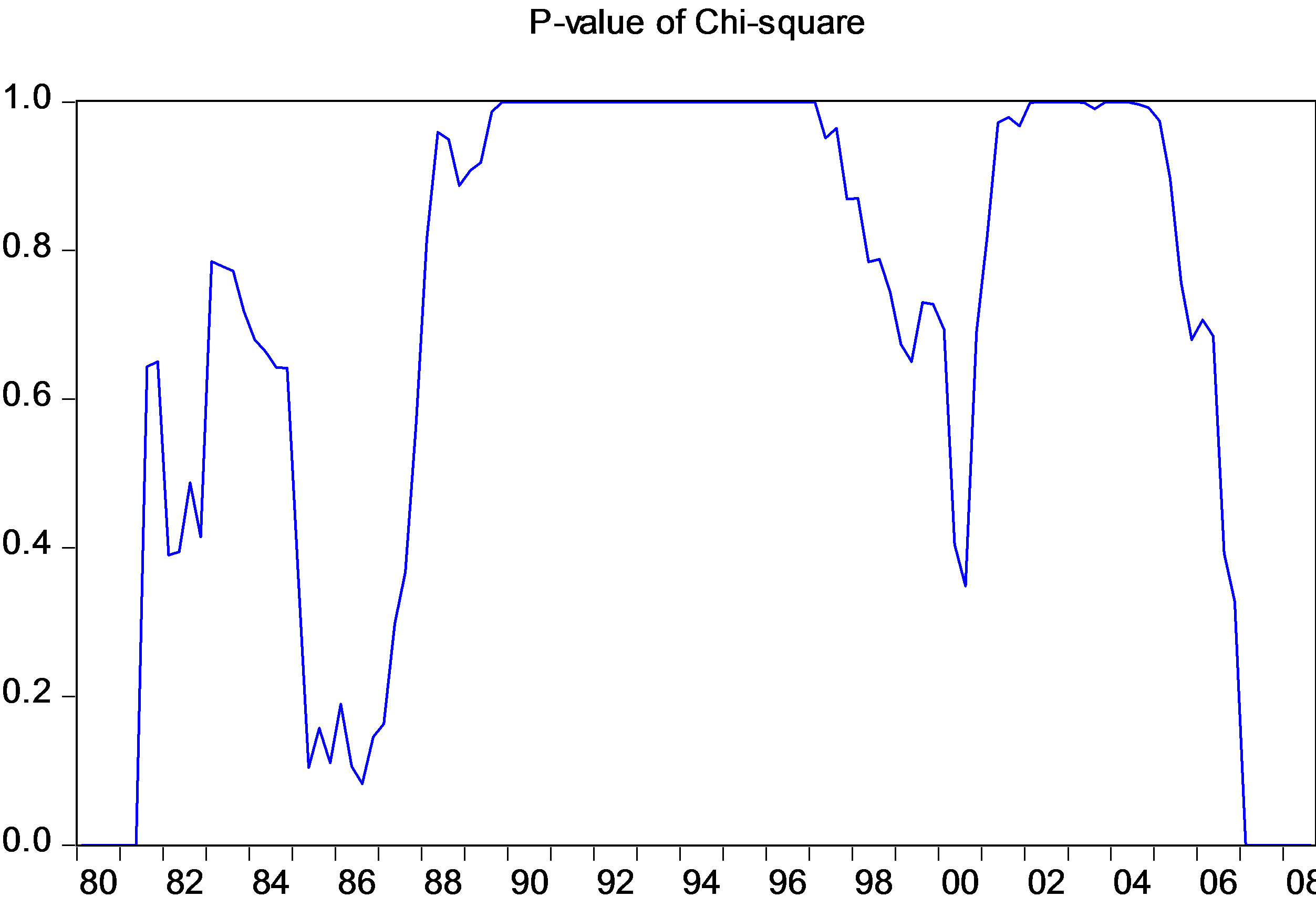
Figure 4. Stability test for VAR with two lags.
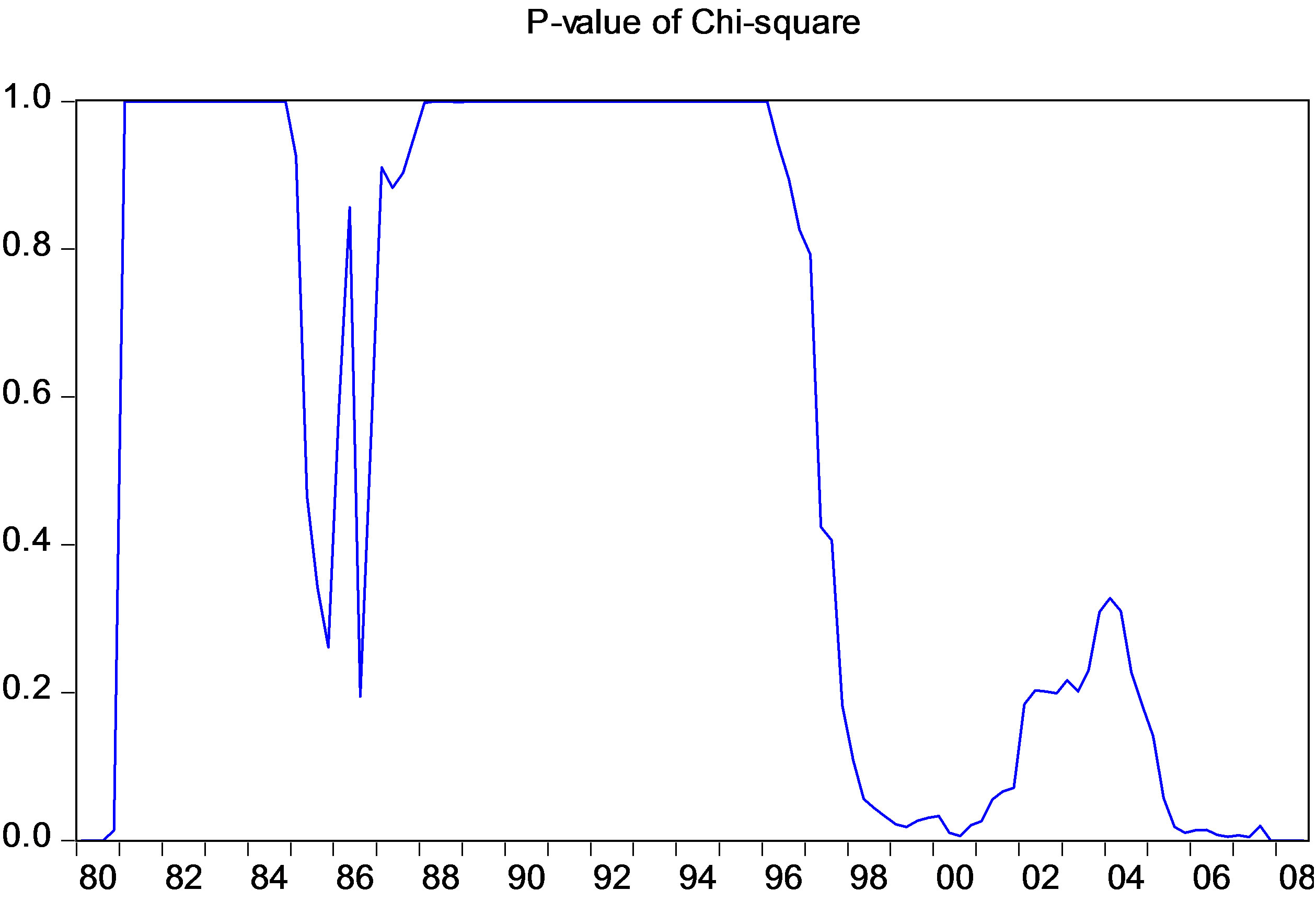
Figure 5. Stability test for VAR with one lag.
nomic environment surrounding Japan changed noticeably around the two break points (1986Q3 in Figure 4 and 2000Q3 in Figure 5). The Japanese yen appreciated dramatically between 1985 and 1986. Also, as illustrated in Figure 1, Japan’s trade volume began to decline in 2000, especially with a sharp decrease in trade with the United States. In contrast, Japan’s trade with China began to sharply increase in 2002.
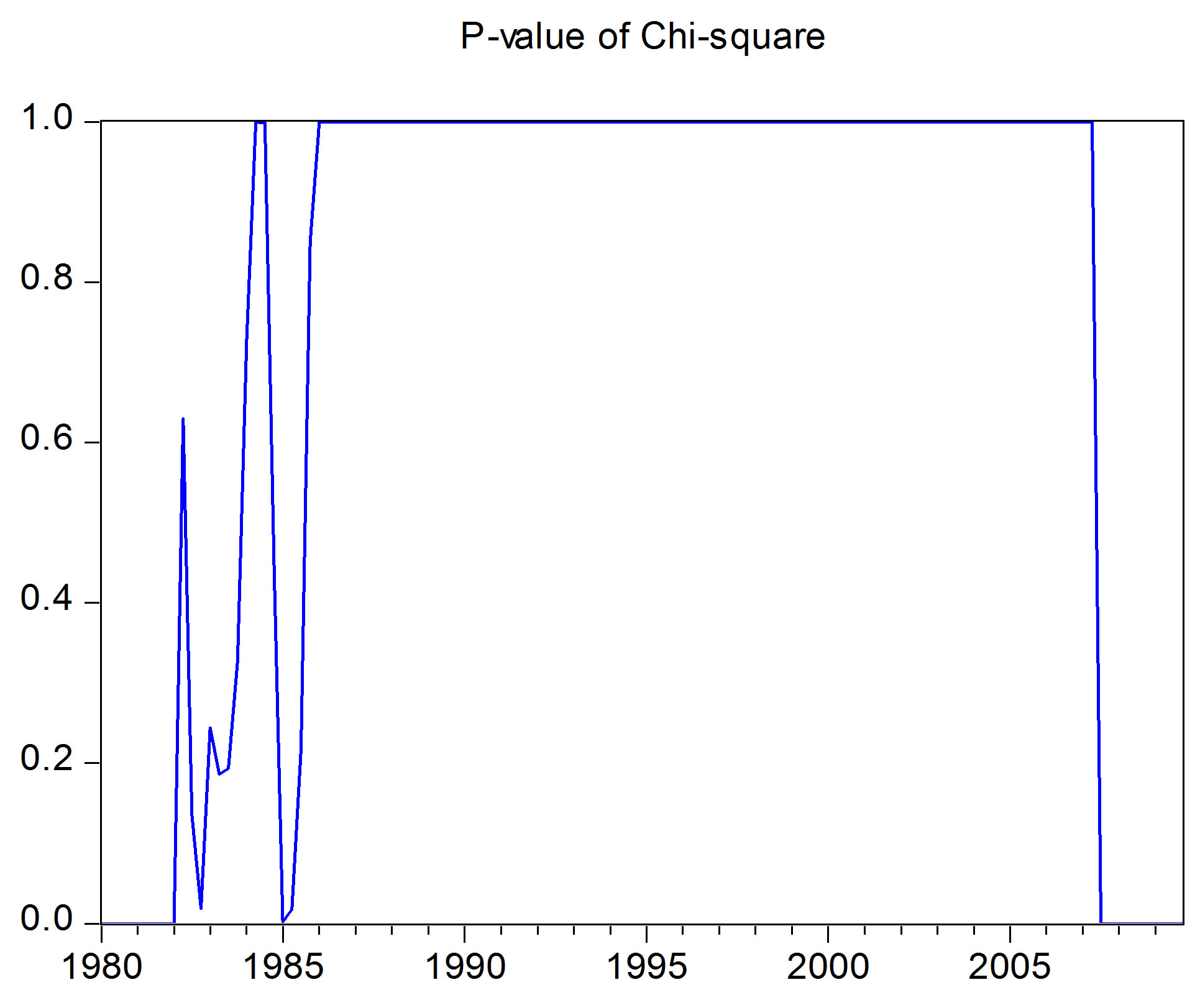
In the Hodrick-Prescott filter, it becomes difficult to accurately divide the variable into trend and cycle parts near the ending point of the sample period. In regard to this, it should be noted that we analyzed the data from 1980Q1 to 2012Q4 at first. But, as shown in Figure 6, the period near the ending point shows high instability. The p-value significantly goes down closer to zero around 2008. Apart from the filter’s ending problem, the global recession sparked by the late-2000s financial crisis may possibly have caused the suggested break near 2008. Therefore, after some experiments, we have excluded the data of the recent crisis period (2008Q4-2012Q4). Although it is interesting to examine the J/S-curve for the late 2000s, we should have a longer sample period beyond 2012Q4 to confirm when the global recession gave rise to a structural break in the curve. Accordingly, we end the sample period at 2008Q3.
2.4. Findings from the Aggregate Trade Data
2.4.1. Aggregate Trade with the Rest of the World
Based on the results from Figures 4, 5, and 6, and considering that there were noticeable changes in the economic environment around the two break points, we divide the whole period into three sub-periods: (a) 1980Q1 ~1986Q2, (b) 1986Q3~2000Q2, and (c) 2000Q3~ 2008Q3. Figures 7 and 8 and Table 4 depict cross-correlations, impulse response functions, and Granger causality tests, respectively, for those three periods.
In Figure 7, the cross-correlations do not appear in the S-shape for period (a). The most S-shaped curve emerges from period (b). In period (c), the S-shape becomes somewhat deformed relative to that in period (b). However, a drop at time 0 has deepened in period (c). In addition, it takes longer in period (c) for the cross-correlation to go up to a zero value after time 0.
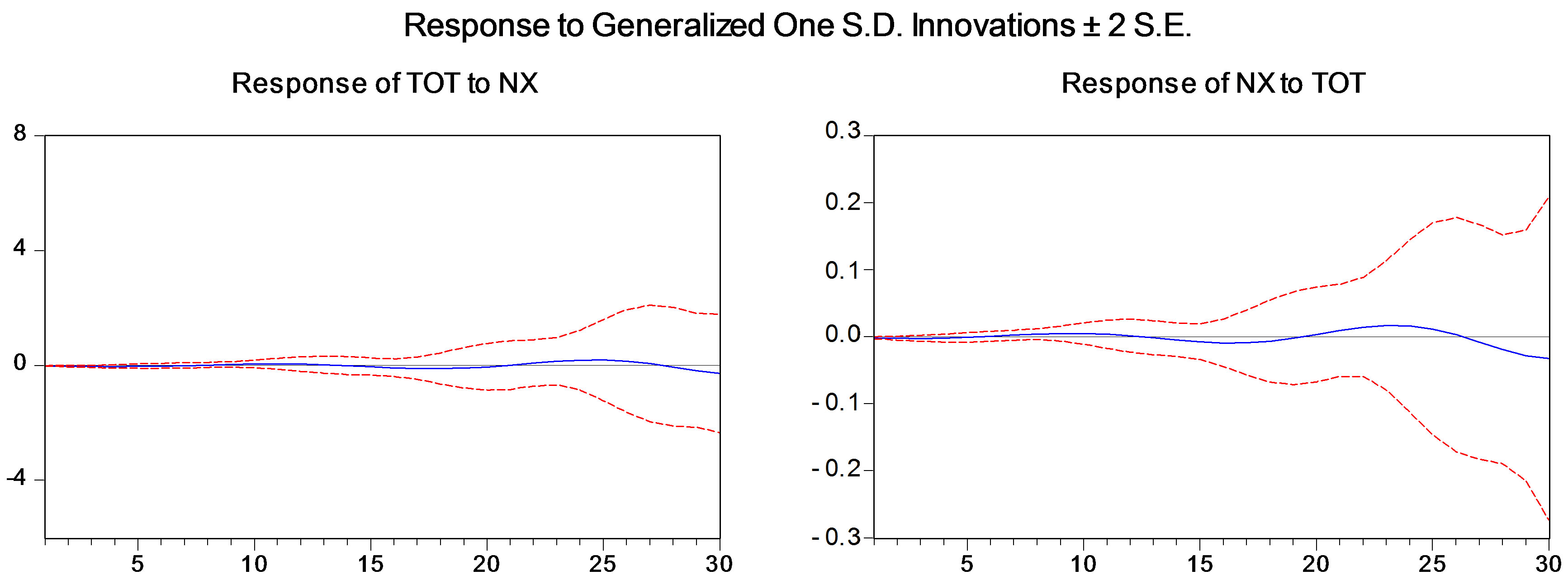
For period (a), the impulse response function of the VAR model does not behave well because of the explosion (see Figure 8(a)). For periods (b) and (c), a response of NX to a shock in the TOT demonstrates the J-curve in both periods, as shown in Figures 8(b) and (c). Similarly, a response of TOT to a shock in the NX produces the right-hand side of the S-curve. One difference between periods (b) and (c) is that an impact of TOT on NX at time 0 has become stronger in the later period. Accordingly, it takes longer in period (c) than in period (b) for the impact to rise beyond the zero level after time 0. This difference is similar to one observed in Figure 7, and it implies that the Japanese economy may have become more vulnerable to a negative external shock.
The Granger causality test results reported in Table 4 show that the null hypothesis of no causality is accepted for both directions in period (a) but is rejected for both directions in periods (b) and (c) at the 5% significance level.

Figure 6. Stability test for VAR for the period from 1980Q1 to 2012Q4 (SIC: Three lags).
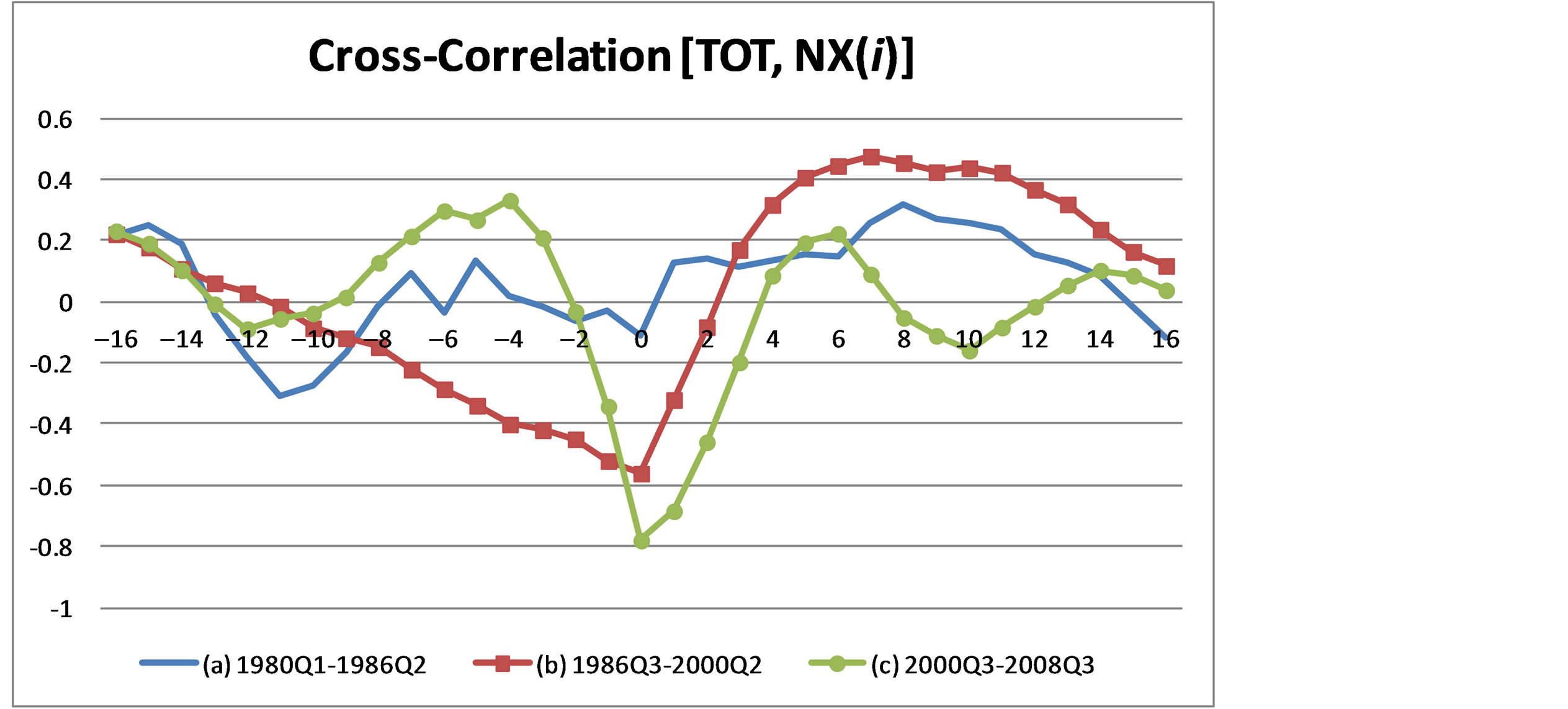
Figure 7. Cross-correlations for periods (a), (b), and (c).
 (a)
(a)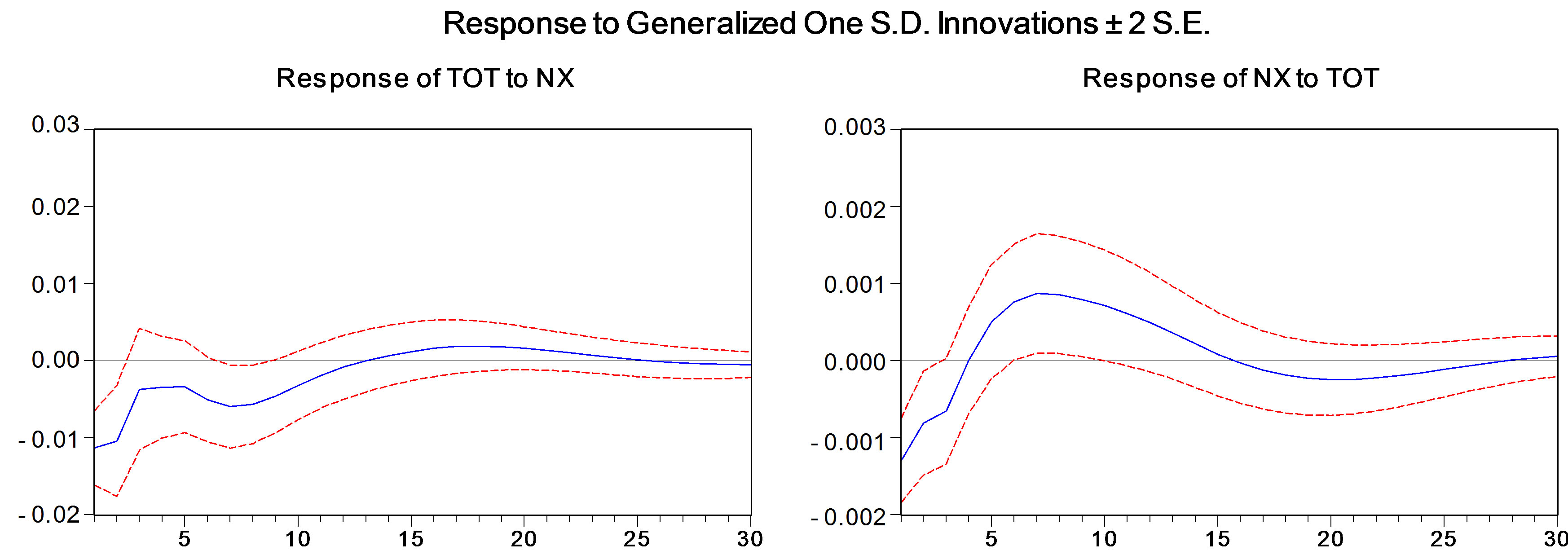 (b)
(b)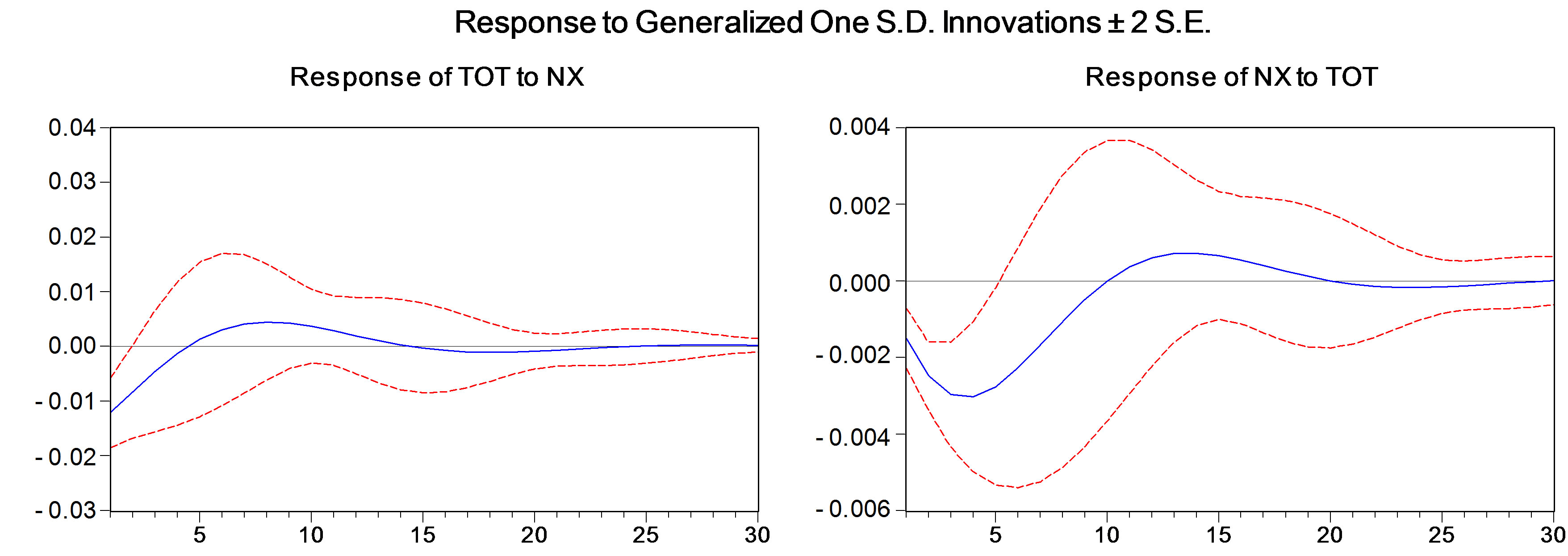 (c)
(c)
Figure 8. (a) 1980Q1-1986Q2 (SIC: Two lags); (b) 1986Q3-2000Q2 (SIC: Three lags); (c) 2000Q3-2008Q3 (SIC: One lag).
Regarding the basic results from these figures and tables, we conclude that the J/S-curve appears in periods (b) and (c) but the shape is not quite the same. For period (a), we cannot reach a clear conclusion about the J/Scurve because of the short length of the time period.
Hereafter, we focus mainly on periods (b) and (c) for two reasons. First, the time length of period (a) is not long enough to generate a meaningful conclusion; second, data for bilateral trade with the advanced country group and China are not completely available during period (a), as will be explained in the following section. For this connection, Figure 9 illustrates cross-correlations between net exports and the terms of trade during periods (b) and (c) combined. We can observe a sharp drop at time 0. Figure 10 illustrates that a response of NX to a shock in the TOT produces the J-curve and that a response of TOT to a shock in NX produces the right-hand side of the S-curve. In Table 5, however, Granger causality tests accept the null hypothesis for both causalities, even at the 10% significance level.
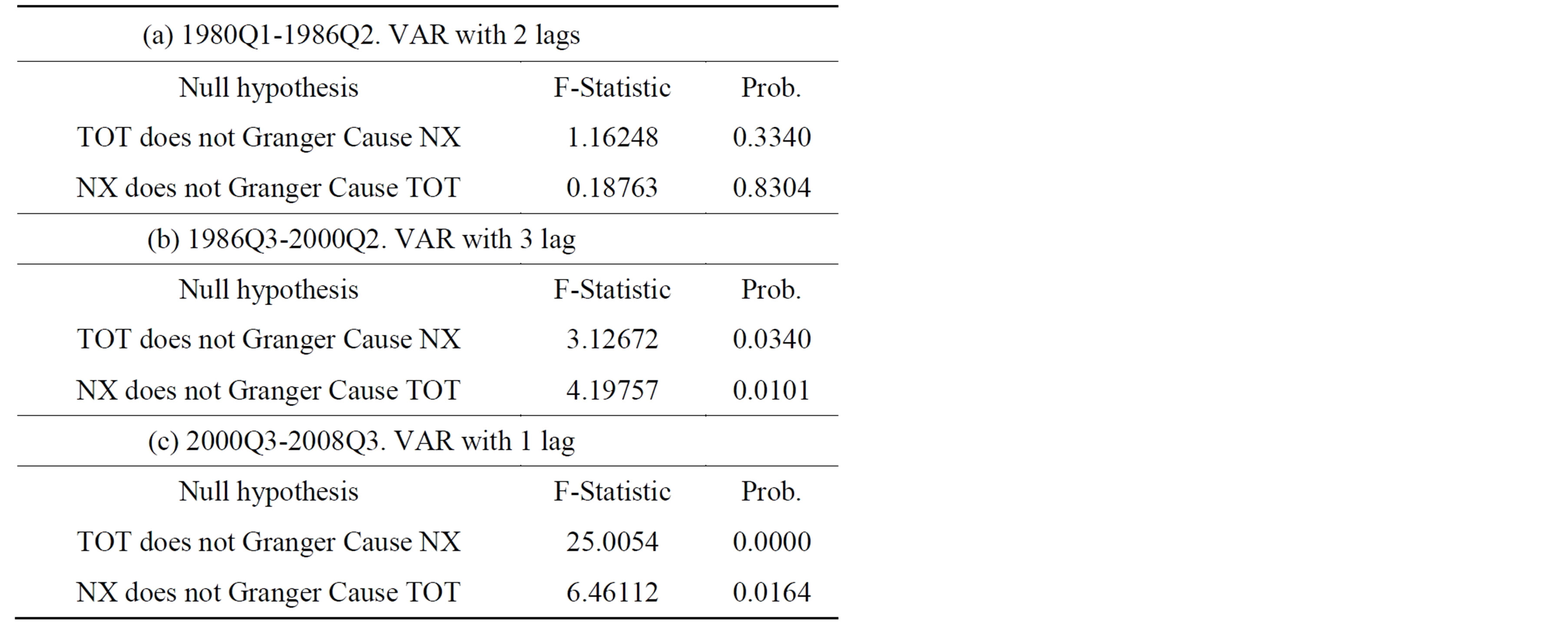
Table 4. Granger causality tests for periods (a), (b), and (c).
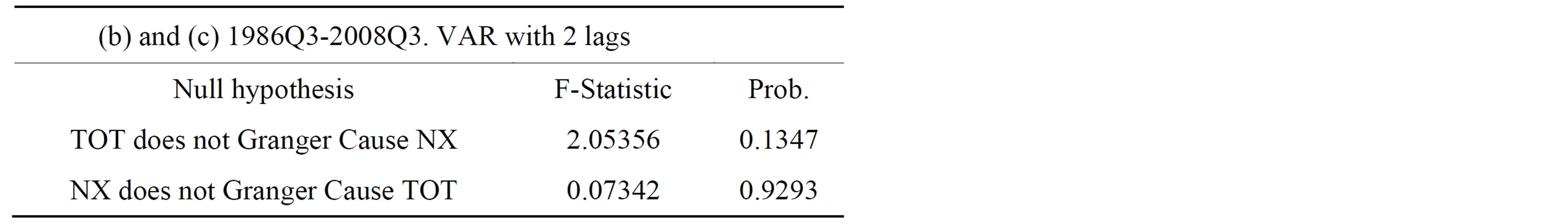
Table 5. Granger causality tests for periods (b) and (c) combined.
2.4.2. Aggregate Trade with Advanced Countries
To examine whether the J/S-curves shown from the aggregate data can also be detected from a subset of the trade data, we also examine Japan’s trade with advanced countries, including the United States and the euro area.
Here, NX denotes Japan’s net exports with advanced economies, the data for which are available from the DOTS. However, TOT is replaced by RELV (real effective exchange rate on unit labor cost for advanced countries), the data for which are available from 1984Q1 in the IFS. In Figure 11, the stability test indicates that the lowest p-value appears to be almost zero at 1989Q2. Figure 12 demonstrates cross-correlations between net exports and the terms of trade (that is, RELV) during a period from 1989Q2 to 2008Q3. Unlike in Figure 9, a negative correlation does not occur at time 0. Figure 13 does not reveal the J-curve phenomenon either. In Table 6, Granger causality tests reject the null hypothesis for both causalities at the 10% significance level. A drop at time 0, observed in Figure 9, may stem from trade with developing countries. With this background, we examine the bilateral trade data in the following section.
3. Analyses of Bilateral Trade Data
In this section we examine the trade and exchange rate data between Japan and its four major trading partners: China, Korea, the United States, and the oil-exporting countries. The oil-exporting countries include Iran, Kuwait, Qatar, Saudi Arabia, and the United Arab Emir
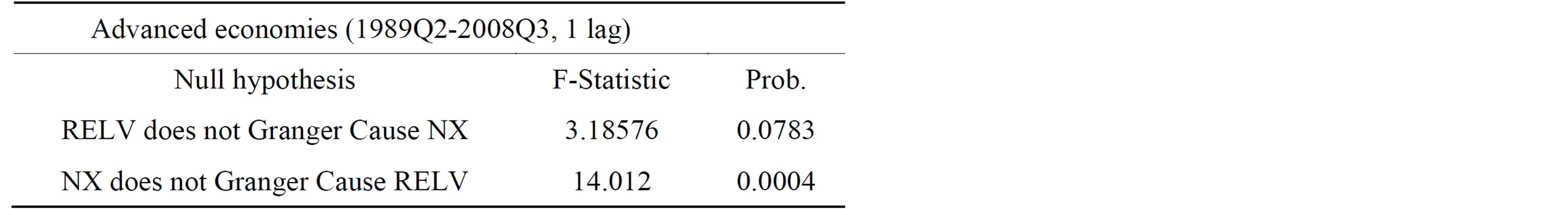
Table 6. Granger causality tests for trade with advanced economies.
ates10. As of 2008, the U.S. market share of Japanese exports was 17.8%, followed by China (16.0%) and Korea (7.6%), and the share of the oil-exporting countries in Japanese exports was 3.17%. On the other hand, the oilexporting countries made up the biggest share (20.7%) of Japan’s imports, followed by China (18.8%), the United States (10.4%), Australia (4.4%), and Korea (3.9%).
Because import and export price data are not available for bilateral trade, the terms of trade used in the previous sections are replaced in this section by real exchange rates computed by nominal exchange rates and consumer price indices for China, Korea, and the United States. On the other hand, for the oil-exporting countries, the terms of trade are computed by the Dubai spot price index divided by the Japanese export price index. The definition of net exports remains the same. Therefore NX still denotes net exports, but RE (real exchange rate) replaces TOT (terms of trade) in this section, except for the oilexporting countries. For notational consistency, the terms of trade between Japan and the oil-exporting countries is also denoted by RE. Because the Chinese consumer price indices are not available before 1986, the Chinese data covers the period from 1986Q1 to 2008Q3; for others, the time periods are the same as in Section 2. As reported in Table 2, the SL unit root tests indicate that the cycle parts of net exports and real exchange rates are stationary, as are those of the aggregate data.
Because structural breaks were detected with the aggregate data in Section 2, the stability test of VAR ([19- 22]) is performed for the whole period in this section, too, to detect possible structural breaks in the relationship between the real exchange rate and trade in each bilateral case. As seen in Figure 14, a statistically significant break at the 10-percent significance level is detected at 1985Q2 with the US data, at 1988Q2 with the Chinese data, and at 2004Q2 with the oil-exporting countries’ data. Although the Korean data do not depict a significant break, some instability is shown at 1986Q3. Considering that no Chinese data are available before 1986 and that the mid-1980s is often detected as a break with the aggregate data and also with some bilateral data, this section excludes the data from 1980Q1 to 1986Q2 for the J-curve analyses with the bilateral data. Further, since
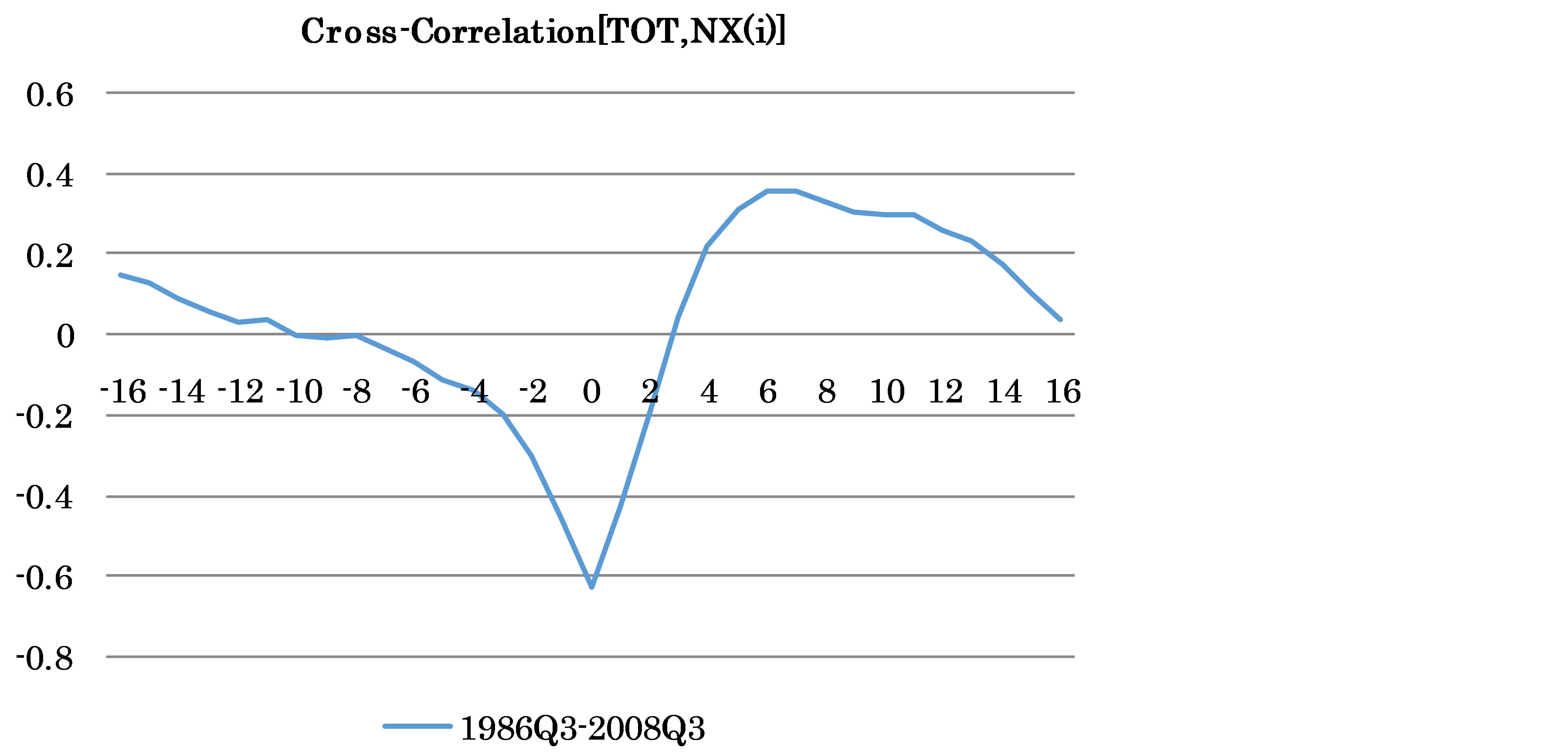
Figure 9. Periods (b) and (c) combined for aggregated trade.
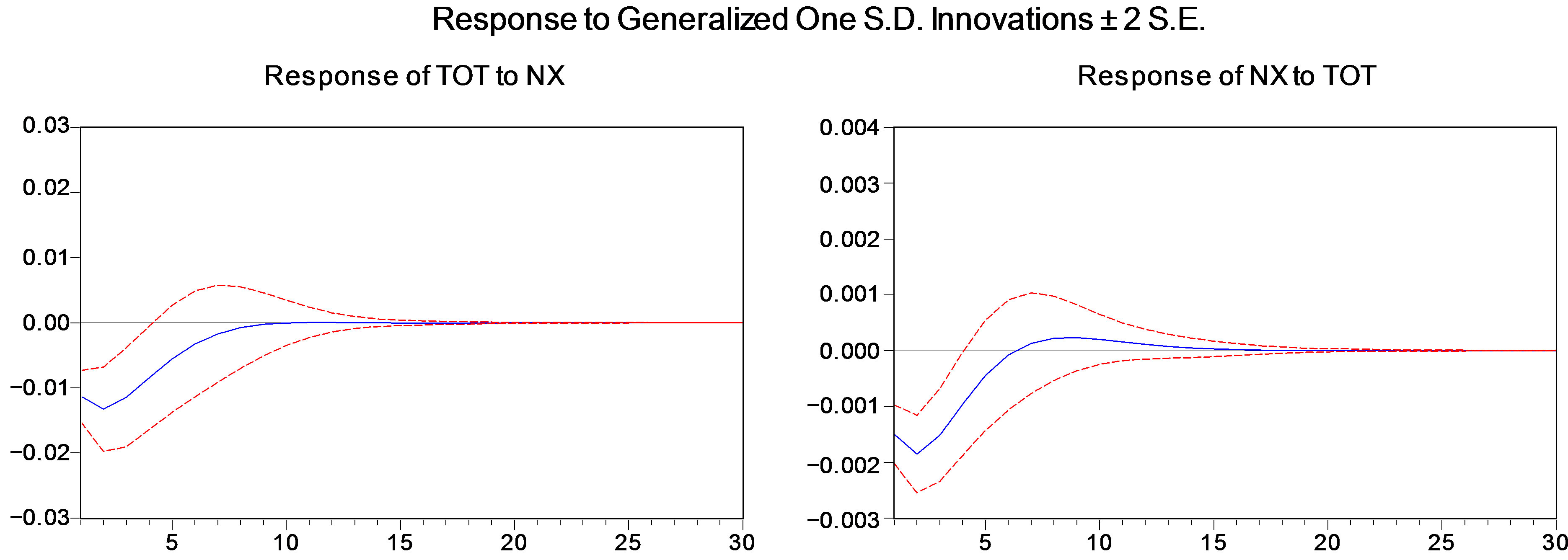
Figure 10. (b) and (c) 1986Q3-2008Q3 (SIC: Two lags).
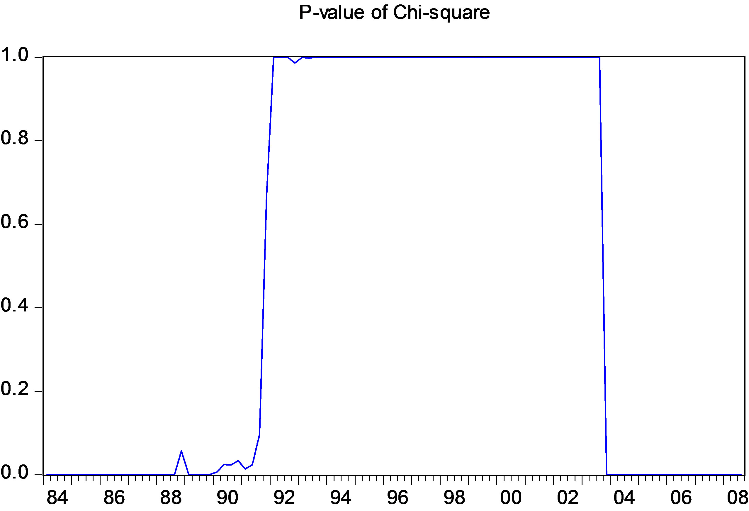
Figure 11. Advanced economies (1984Q1-2008Q3, SIC: One lag).
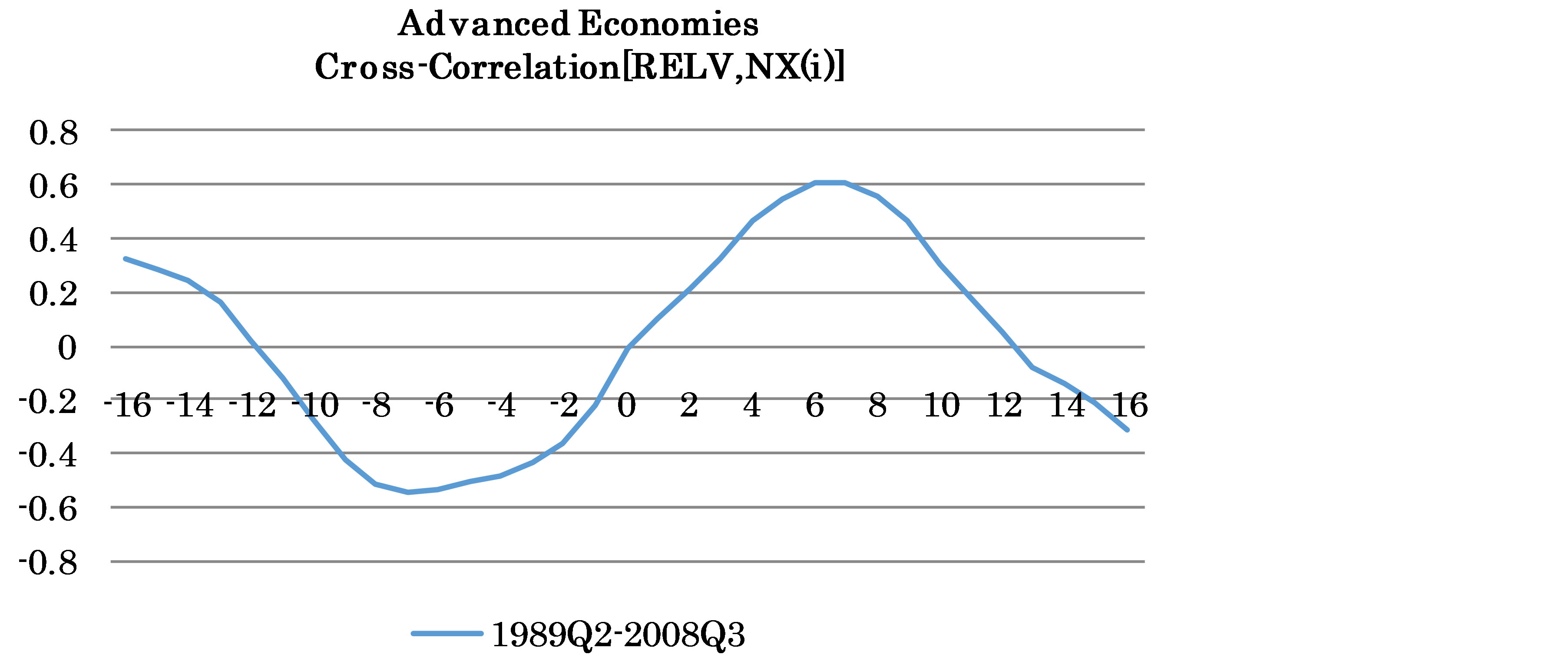
Figure 12. Cross-correlations for trade with advanced economies.
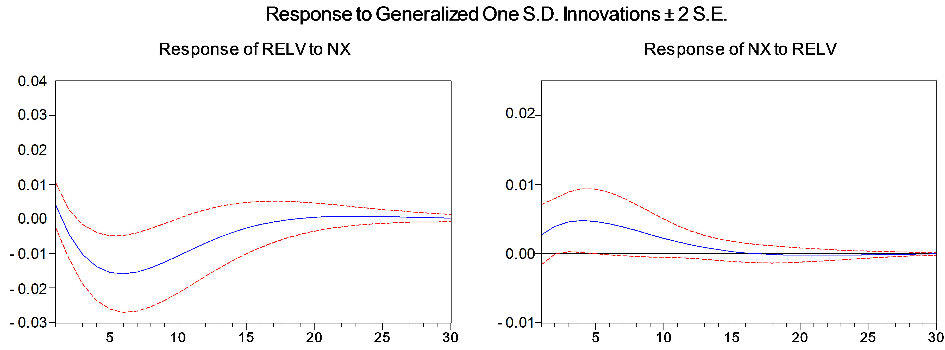
Figure 13. Advanced economies.
the detected break is at 1988Q2 for China, the Chinese data are analyzed only for after 1988Q2. Even though the previous section split the aggregate data into two sub-periods (1986Q3-2000Q2 and 2000Q3-2008Q3) since 1986Q3, the bilateral data are not split in the same way, because no bilateral data imply 2000 as a break. In summary, the J-curve analyses with the bilateral data in this section are performed for the following time periods: China from 1988Q3 to 2008Q3; and Korea, the United States, and the oil-exporting countries from 1986Q3 to 2008Q3.
3.1. Cross-Correlations
As seen in Figures 15(a) through (d), the cross-correlation coefficients between RE (real exchange rate) and NX (net exports) illustrate somewhat different dynamics across the trading partners of Japan. Among them, the data of Korea and the United States do not show the Jcurve that was shown with the aggregate data for the same time period. In contrast, the data of China and the oil-exporting countries demonstrate the J-curve. Considering that the share of China and the oil-exporting countries in Japanese trade has increased for the last few decades, as shown in Figure 1, the preceding findings can be regarded as implying that the J-curve shown in the aggregate data is the result of increasing influences of China and the oil-exporting countries on Japanese external trade. The finding in Section 2—that the bilateral data for the advanced countries for the period from 1989Q2 to 2008Q3 do not display the J-curve—implies the same. Moreover, Section 2 reports that the aggregate data do not display a J-curve for the period before 1986Q3, whereas they show a J-curve for the period after 1986Q3. In other words, the aggregate data do not show a J-curve when the advanced countries have a higher share of Japanese trade, but do show a J-curve when China and the oil-exporting countries have a higher share.
It should be also noted that the correlation coefficient at time 0 is much lower in the case of the oil-exporting countries (Figure 15(d)) than in the case of China (Figure 15(c)). Also of interest, the same coefficient of
 (a)
(a) (b)
(b)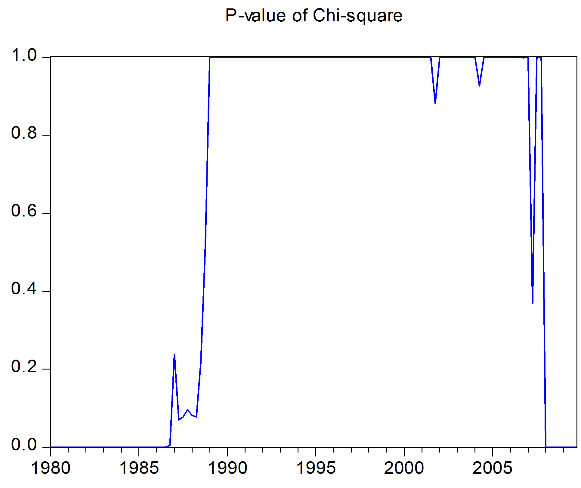 (c)
(c)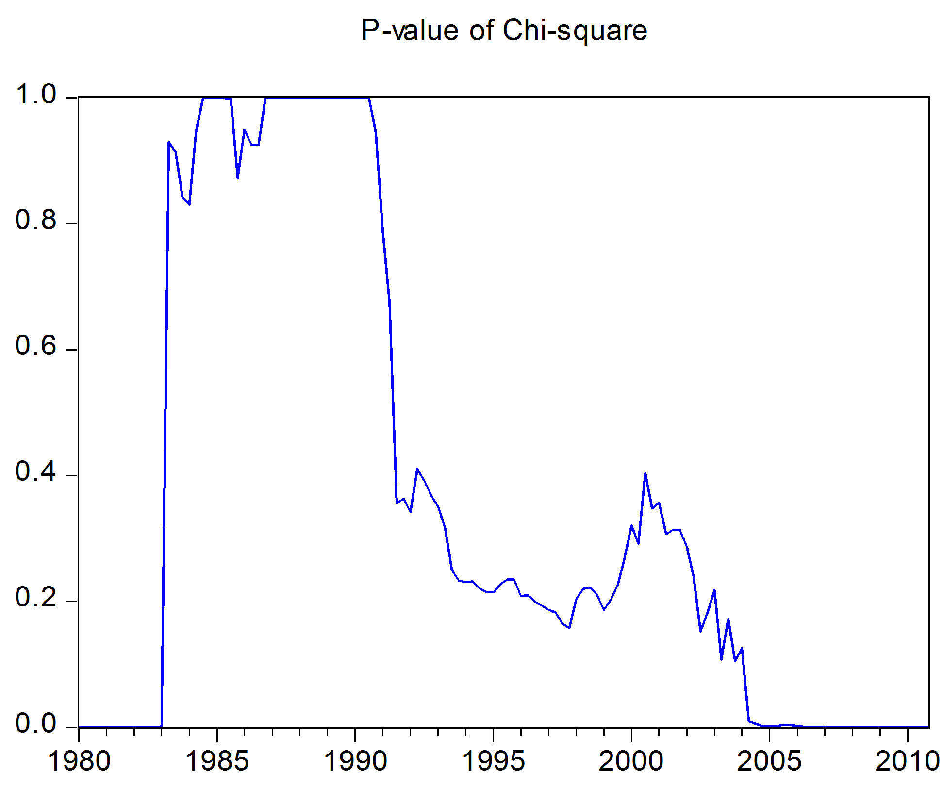 (d)
(d)
Figure 14. VAR stability test for bilateral data; (a) US data; (b) Korean data; (c) Chinese data; (d) Oil-Exporting countries data.
the aggregate data in Figure 7 is lower in period (c) from 2000Q3 to 2008Q3 than in period (b) from 1986Q3 to 2000Q2. Considering that the share of the oil-exporting countries sharply increased in period (c), it is not surprising that the J-curve in period (c) exhibits a pattern similar to the J-curve of the oil-exporting countries. This finding also implies that the changing shares in Japanese trade might lead to the changes in the forms of the Japanese J-curve.
3.2. Impulse Responses and Granger Causality
In this part, the relationship between exchange rates and trade balance is examined by impulse responses and Granger causality tests. The lag length of VAR models is determined by SIC, just as in Section 2.
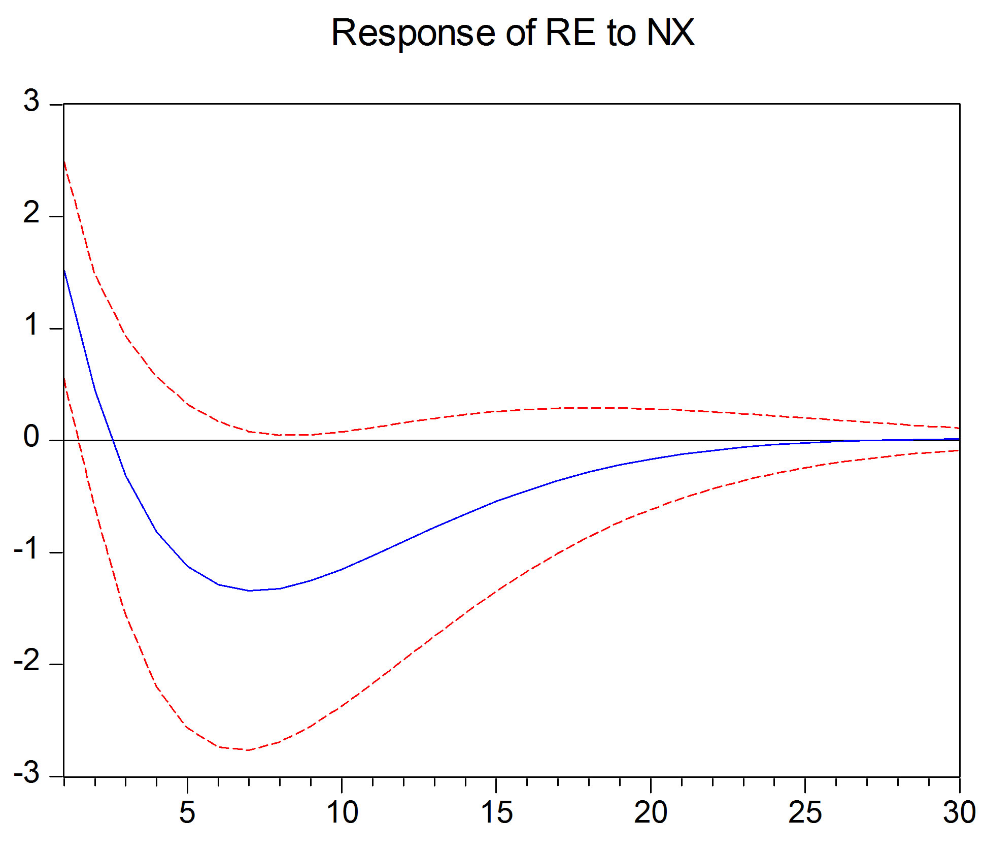
As shown in Figures 16(a) and (b), the impulse responses of the United States and Korea do not show the J-curve phenomenon that is shown in the aggregate data for periods (b) and (c) in Figures 8(b) and (c). In contrast, the impulse responses of China and the oil-exporting countries in Figures 16(c) and 16(d) show a J-curve phenomenon similar to those of the aggregate data. Moreover, as in the case with the cross-correlations analyzed in the previous section, impulse responses of the data of the oil-exporting countries show dynamics similar to those of the aggregate data in period (c), in which the share of oil-exporting countries sharply increased.
In the meantime, the Granger causality test results reported in Table 7 show that no bilateral case generates the same results as those for the aggregate data reported in Table 4. In Table 4, TOT turns out to Granger-cause
 (a)
(a)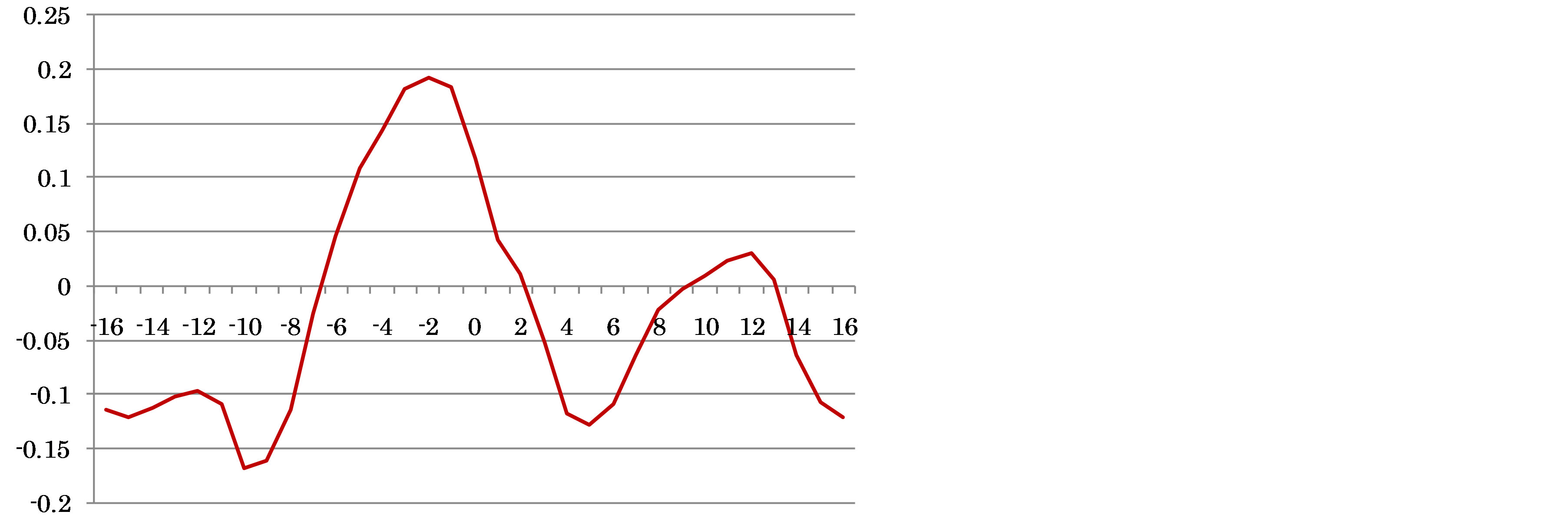 (b)
(b)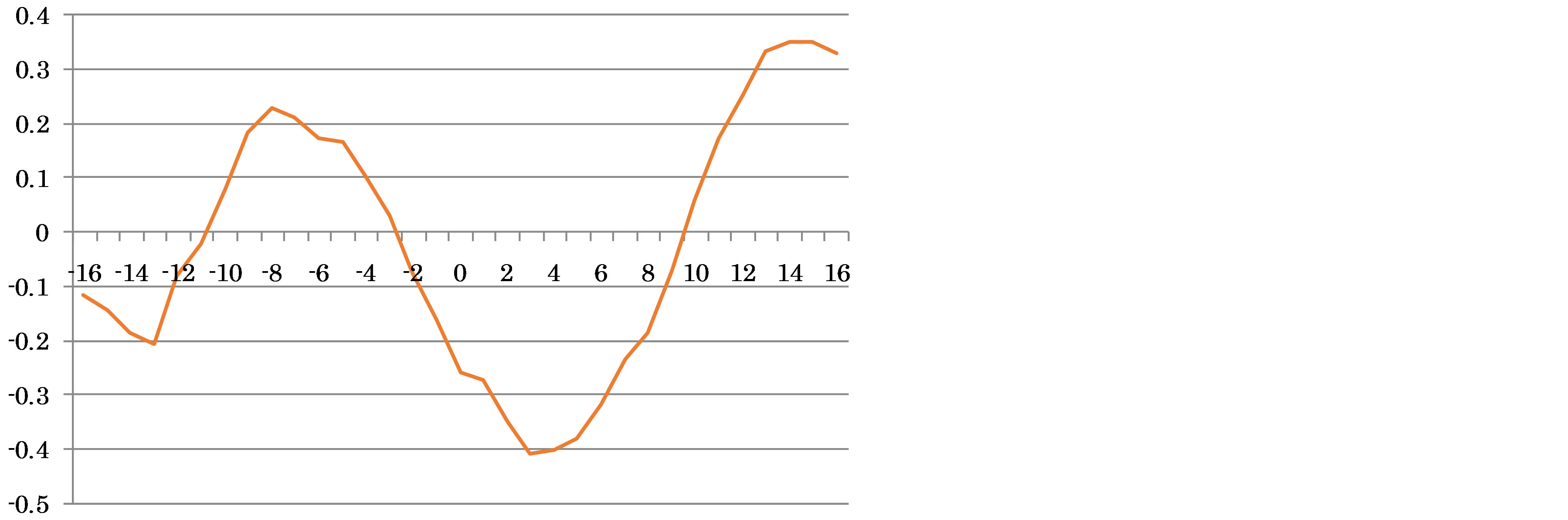 (c)
(c) (d)
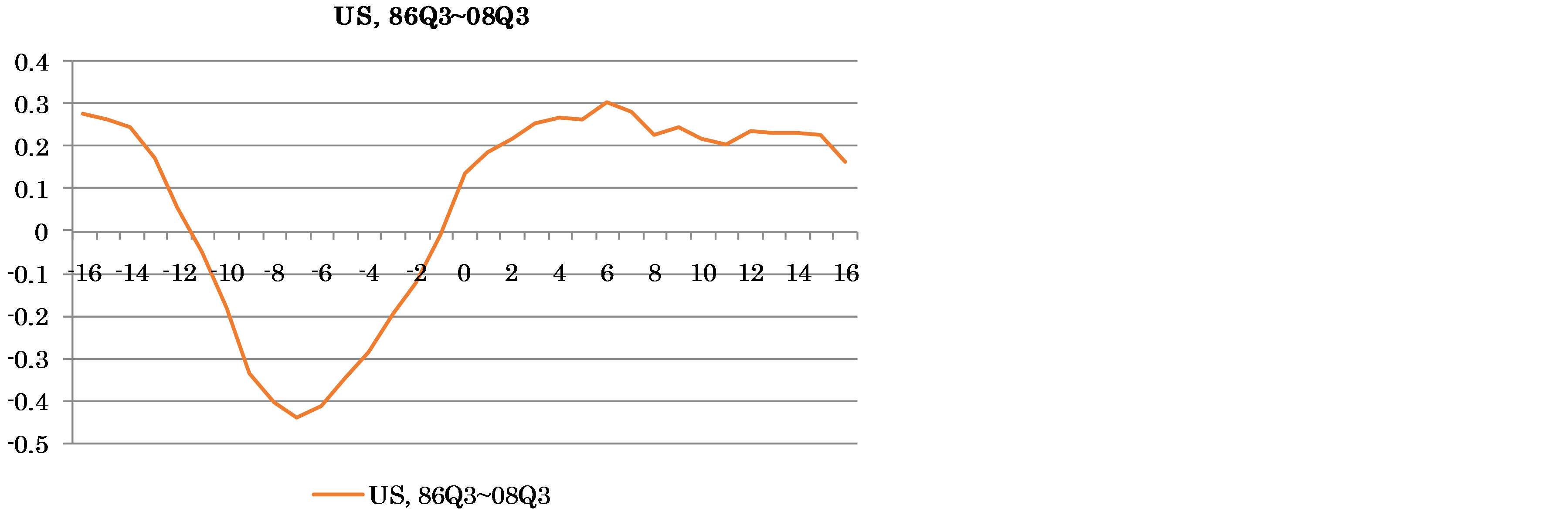
(d)
Figure 15. (a) Cross-correlations of the US data (Period: 86Q3-08Q3); (b) Cross-correlations of the Korean data (Period: 86Q3-08Q3); (c) Cross-correlations of the Chinese data (88Q4-08Q3); (d) Cross-Correlations of the Oil-Exporting countries’ data (86Q3-08Q3).
in period (b) at the 5-percent significance level and in period (c) even at the 1-percent significance level. NX Granger-causes TOT at the 5-percent significance level in periods (b) and (c).
In Table 7, neither RE nor NX Granger-cause the other with the data of China. With the data of Korea and the United States, NX Granger-causes TOT, but TOT does not Granger-cause NX. With the data of the oil-exporting countries, RE Granger-causes NX, but NX does not Granger-cause RE. Strong causality from TOT to NX with the aggregate data in period (c) is consistent with the same strong causality with the data of the oil-exporting countries. At the same time, causality from NX to TOT with the aggregate data in periods (b) and (c) is consistent with the same causality with the data of Korea and the United States.
4. Conclusions
This paper analyzed Japanese trade balances, terms of trade, and exchange rates for the period from 1980Q1 to 2008Q3 to investigate how Japanese trade balances relate to changes in terms of trade and real exchange rates. In particular, this paper examined whether Jand S-curves
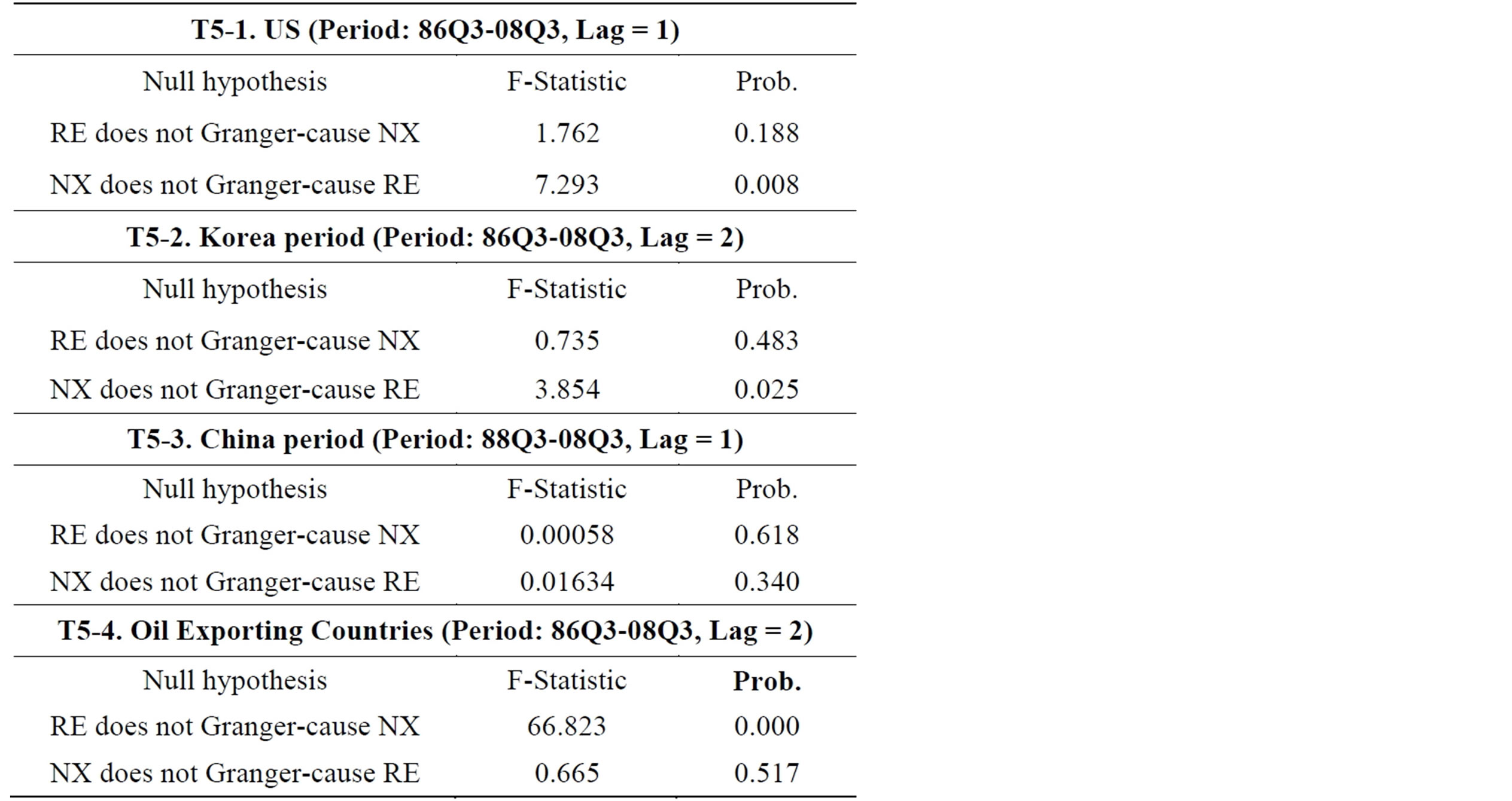
Table 7. Granger causality tests for bilateral data.
were detected in the Japanese economy for the past three decades and whether there were structural breaks in the curves.
 (a)
(a)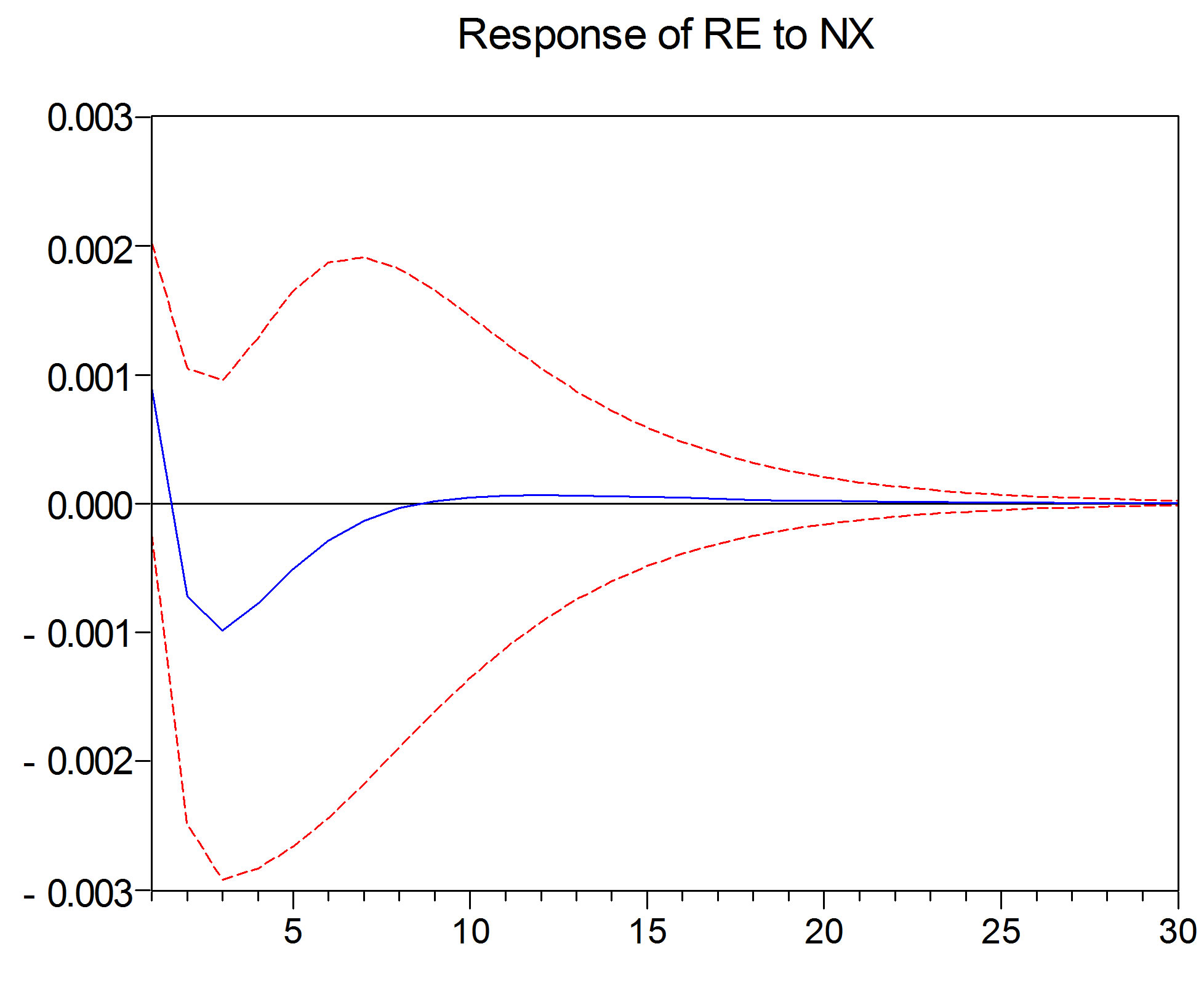 (b)
(b)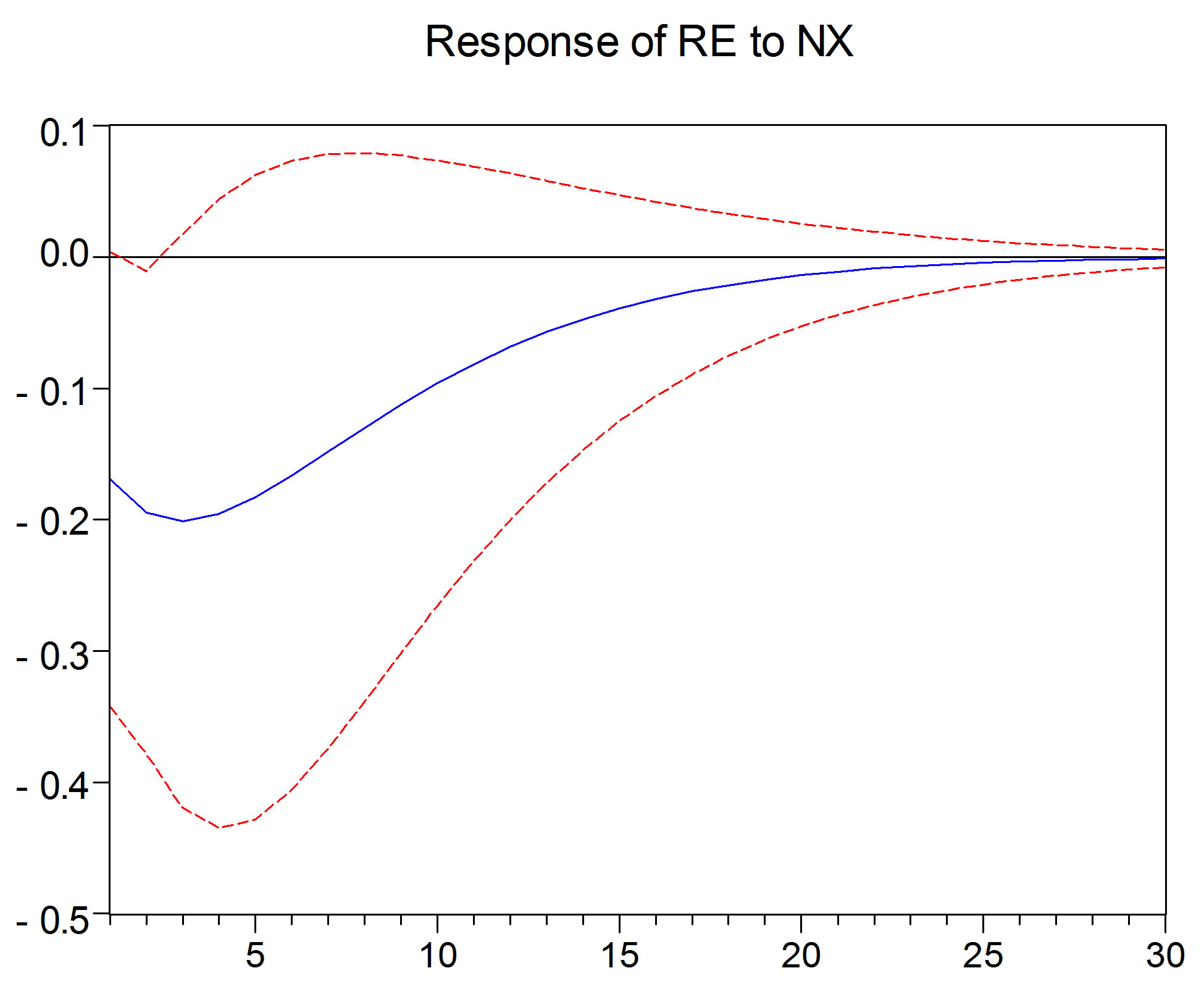 (c)
(c)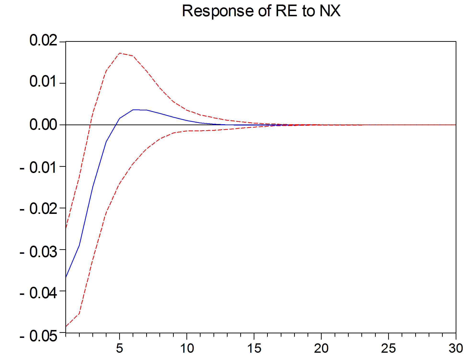 (d)
(d)
Figure 16. (a) Impulse Responses for the US Data (Period: 86Q3-08Q3); RE: Cycle parts of real exchange rates between Japan and the United States; NX: Cycle parts of trade balance between Japan and the United States. (b) Impulse Responses for the Korean Data (Period: 86Q3-08Q3); RE: Cycle parts of real exchange rates between Japan and Korea; NX: Cycle parts of trade balance between Japan and Korea. (c) Impulse Responses for the Chinese Data (Period: 88Q3-08Q3); RE: Cycle parts of real exchange rates between Japan and China; NX: Cycle parts of trade balance between Japan and China. (d) Impulse Responses for the Oil-Exporting Countries’ Data (Period: 86Q3-08Q3); RE: Cycle parts of the terms of trade between Japan and oil-exporting countries; NX: Cycle parts of trade balance between Japan and oil-exporting countries.
To detect structural breaks, VAR stability tests were performed. Because the VAR stability tests implied 1986Q3 and 2000Q3 to be possible structural breaks, the data were split into three sub-periods: period (a) (1980Q1- 1986Q2), period (b) (1986Q3-2000Q2), and period (c) (2000Q3-2008Q3). Computations and test results with aggregate data exhibited the J/S-curves for periods (b) and (c).
Next, the same computations and tests were performed with bilateral trade and exchange rate data between Japan and its four major trading partners: China, Korea, the United States, and the oil-exporting countries. Partly because the Chinese data are not available before 1986, and because significant breaks were rarely detected since the mid-1980s, the bilateral data were analyzed for the period from 1986Q3 to 2008Q3 for Korea, the United States, and the oil-exporting countries and for the period from 1988Q3 to 2008Q3 for China.
Cross correlations did not show the J/S-curve for Japan’s trade with Korea or with the United States, but did show it for Japan’s trade with China and with the oilexporting countries. Of interest is that the J/S-curve of the oil-exporting countries has a pattern similar to that of the aggregate data for period (c), in which the share of the oil-exporting countries had sharply increased. Impulse responses also showed similar dynamics.
Different from cross-correlations and impulse responses, no bilateral data showed the same Granger causality test results with the aggregate data in general. However, a strong causality from RE to NX with the data of the oil-exporting countries is consistent with the same causality with the aggregate data in period (c).
Overall, the findings of this paper imply that the presence of the J/S-curve in the aggregate trade data of Japan in recent periods should be the result of the increasing share of China and the oil-exporting countries in Japanese trade. The share of the oil-exporting countries is affected by oil price changes. Thus the J/S-curve of Japan will be also affected by oil price changes. In the meantime, as China’s share of Japanese trade increases, the relationship between bilateral trade and bilateral exchange rates with China will be an important factor in determining the overall pattern of the relationship in the aggregate data.
Acknowledgements
Previous versions of this paper have been presented at the 2010 Autumn Meeting of the Japanese Economic Association and the 2011 Spring Meeting of the Japan Society of Monetary Economics. The authors would like to thank EtsuroShioji, Sadayoshi Takaya, and the other participants at these meetings for their comments and suggestions. We are supported by the TCER’s individual research grant in 2009 and in part by Grant-in-Aids for Scientific Research (Nos. 19530195, 21530237, and 23530357).
REFERENCES
- S. P. Magee, “Currency Contracts, Pass Through and Devaluation,” Brookings Papers on Economic Activity, Vol. 1, 1973, pp. 303-325. http://dx.doi.org/10.2307/2534091
- M. Bahmani-Oskooee and A. Ratha, “The J-Curve: A Literature Review,” Applied Economics, Vol. 36, 2004, pp. 1377-1398. http://dx.doi.org/10.1080/0003684042000201794
- D. K. Backus, P. J. Kehoe and F. E. Kydland, “Dynamics of the Trade Balance and the Terms of Trade: The JCurve?” American Economic Review, Vol. 84, 1994, pp. 84-103.
- Economic Planning Agency, “Annual Report on Japan’s Economy,” 1986. http://wp.cao.go.jp/zenbun/keizai/index.html
- T. Moriguchi, “Structural Adjustments in the Japanese Economy and Macroeconomic Balance: A Possibility of the Policy Coordination,” Financial Review, Vol. 9, 1989. http://www.mof.go.jp/f-review/r09/r09.htm
- Economic Planning Agency, “Annual Report on Japan’s Economy,” 1997. http://wp.cao.go.jp/zenbun/keizai/index.html
- A. Gupta-Kapoor and U. Ramakrishnan, “Is There a JCurve? A New Estimation for Japan,” International Economic Journal, Vol. 13, 1999, pp. 71-79. http://dx.doi.org/10.1080/10168739900080029
- C. Jung and K. Doroodian, “The Persistence of Japan’s Trade Surplus,” International Economic Journal, Vol. 12, 1998, pp. 1-25.
- M. Noland, “Japanese Trade Elasticities and the J-Curve,” Review of Economics and Statistics, Vol. 71, 1989, pp. 175-179. http://dx.doi.org/10.2307/1928067
- M. Bahmani-Oskooee and G. G. Goswami, “Disaggregated Approach to Test the J-Curve Phenomenon: Japan versus her Major Trading Partners,” Journal of Economics and Finance, Vol. 27, 2003, pp. 102-113. http://dx.doi.org/10.1007/BF02751593
- M. Bahmani-Oskooee and A. Ratha, “Bilateral S-Curve between Japan and Her Trading Partners,” Japan and the World Economy, Vol. 19, 2007, pp. 483-489. http://dx.doi.org/10.1016/j.japwor.2006.09.005
- M. H. Hsing, “Re-Examination of J-Curve Effect for Japan, Korea, and Taiwan,” Japan and the World Economy, Vol. 17, 2005, pp. 43-58. http://dx.doi.org/10.1016/j.japwor.2003.10.002
- M. Kumagai, M. Hashimoto, T. Saito and S. Kugo, “Assessment of Abenomics: Examination of Current Situation and Future Issues,” Japan’s Economic Outlook (Daiwa Institute of Research Group), No. 177, 2013. http://www.dir.co.jp/english/research/report/jquarterly/20130603_007270.pdf
- M. Bahmani-Oskooee and A. Ratha, “S-Curve Dynamics of Trade between US and China,” China Economic Review, Vol. 21, 2010, pp. 212-223. http://dx.doi.org/10.1016/j.chieco.2009.06.006
- P. Perron, “Dealing with Structural Breaks,” In: K. Patterson and T. C. Mills, Eds., Palgrave Handbook of Econometrics, Vol. 1, Econometric Theory, Palgrave, London, 2006.
- P. Saikkonen and H. Lutkepohl, “Testing for a Unit Root in a Time Series with a Level Shift at Unknown Time,” Econometric Theory, Vol. 18, 2002, pp. 313-348. http://dx.doi.org/10.1017/S0266466602182053
- M. Lanne, H. Lutkepohl and P. Saikkonen, “Comparison of Unit Root Tests for Time Series with Level Shifts,” Journal of Time Series Analysis, Vol. 23, 2002, pp. 667- 685. http://dx.doi.org/10.1111/1467-9892.00285
- H. H. Pesaran and Y. Shin, “Generalized Impulse Response Analysis in Linear Multivariate Models,” Economics Letters, Vol. 58, 1998, pp. 17-29. http://dx.doi.org/10.1016/S0165-1765(97)00214-0
- C. Sims, “Macroeconomics and Reality,” Econometrica, Vol. 48, 1980, pp. 1-48. http://dx.doi.org/10.2307/1912017
- L. J. Christiano, “Money and the US Economy in the 1980s: A Break from the Past,” Quarterly Review, Vol. 10, 1986, pp. 2-13.
- S. Cecchetti and G. Karras, “Sources of Output Fluctuations during the Interwar Period: Further Evidence on the Causes of the Great Depression,” Review of Economic Statistics, Vol. 76, 1994, pp. 80-102. http://dx.doi.org/10.2307/2109828
- R. Miyao, “Time-Series Analysis on the Macroeconomic Monetary Policy,” Nihon-Keizai Shimbun-sha, Tokyo, 2006.
- G. W. Snedecor and W. G. Cochran, “Statistical Methods 7,” 6th Edition, Translated into Japanese by M. Hatamura, T. Okuno and Y. Tsumura, Iwanami-Shoten, Tokyo, 1972.
- Y. Kano, “Lecture’s FAQ Page 1,” 2004. http://bm.hus.osaka-u.ac.jp/~kano/lecture/faq/q1.html
- IEEJ, “2010 Oil Now,” The Institute of Energy Economics, 2010. http://eneken.ieej.or.jp/en/
NOTES
*Corresponding author.
1The numbers in this and the following paragraph were computed with data obtained from the Direction of Trade Statistics (DOTS) and the International Financial Statistics (IFS) of the International Monetary Fund (IMF), unless otherwise stated.
2The exchange rate was 257.68 yen at 1985Q1, 153.17 yen at 1987Q1, and 128.45 yen at 1989Q1.
3The exchange rate was 84.43 yen at 1995Q2 and 121.22 yen at 1997Q1.
4See also [7-9].
5The averaged monthly exchange rate of the yen against a dollar went from 80.92 yen in November 2012 to 101.01 yen in May 2013 (according to the data from the Bank of Japan).
6Using the data from the 1970s to the 1990s, [10] reports no evidence for structural changes in most of their estimations regarding the J curve.
7A more detailed explanation is provided in Subsection 2.3.
8See [18] for details, and [12] for its application to the J curve.
9For an equality test between two ordinary correlations, see [23,24]. One may want apply their method to an equality test between two cross-correlations.
10According to [25], Japan imported 82.2 percent of its oil from those countries in 2009.