Wireless Engineering and Technology
Vol.3 No.3(2012), Article ID:21466,4 pages DOI:10.4236/wet.2012.33020
Analyzing History Quality for Routing Purposes in Opportunistic Network Using Max-Flow
![]()
1Faculty of Computer Sciences and Engineering, GIK Institute, Topi, Pakistan; 2Distributed Systems Laboratory, University of Konstanz, Konstanz, Germany.
Email: arshad.islam@giki.edu.pk, marcel.waldvogel@uni-konstanz.de
Received March 8th, 2012; revised April 4th, 2012; accepted May 9th, 2012
Keywords: Opportunistic Networks; Delay Tolerant Networks; Routing Protocols; Max-Flow; Simulation; Modified Dijk-Stra Algorithm
ABSTRACT
Most of the existing opportunistic network routing protocols are based on some type of utility function that is directly or indirectly dependent on the past behavior of devices. The past behavior or history of a device is usually referred to as contacts that the device had in the past. Whatever may be the metric of history, most of these routing protocols work on the realistic premise that node mobility is not truly random. In contrast, there are several oracles based methods where such oracles assist these methods to gain access to information that is unrealistic in the real world. Although, such oracles are unrealistic, they can help to understand the nature and behavior of underlying networks. In this paper, we have analyzed the gap between these two extremes. We have performed max-flow computations on three different opportunistic networks and then compared the results by performing max-flow computations on history generated by the respective networks. We have found that the correctness of the history based prediction of history is dependent on the dense nature of the underlying network. Moreover, the history based prediction can deliver correct paths but cannot guarantee their absolute reliability.
1. Introduction
Since the initial introduction of Delay Tolerant Networks on the research horizon for interplanetary communication [1], several offshoots have spawned, e.g. Vehicular Networks, Mobile Social Networks and Opportunistic Networks. Similarly, several practical applications, such as an emergency response in case of a catastrophe, military operations and non-interactive Internet access in rural areas [2] have vastly increased the usability of such networks. Although, there have been a few practical deployments of opportunistic networks [3,4], simulation is still the favorite tool assisting us in analyzing opportunistic networks with several variations, e.g. mobility pattern of devices, variable bandwidth, obstacles and other environmental effects.
The challenges involved in opportunistic network routing are totally different from the traditional wired networks. We cannot only design and plan the structure of wired networks, but in case part of a network fails, we receive real time information about the route changes in the network. On the other hand, opportunistic networks (as the name suggests) cannot be designed or planned. They are implicitly created and evolve due to wireless devices that come into each other’s radio range. These wireless devices then behave as data mules as well as routers. They make routing decisions to bring the messages to their respective destinations based on the local knowledge that they have obtained earlier from the network.
One of the not that obvious effect of delay in Opportunistic Networks is lack of accurate information flow. Due to intermittent connectivity, a node that may be temporarily connected to a cluster, is not able to advertise its new contacts. By the time potential consumers get the access to this info, it is outdated and that edge may not be available anymore. This problem becomes two fold when we incorporate the congestion factor into the scenario. In traditional networks, congestion related information is available in accurate and timely fashion. As soon as, an edge gets congested, appropriate measures like exponential back off are taken immediately. In the case of opportunistic networks, delay destroys this promise of congestion handling and avoidance. Ideally, we would like to distribute congestion related information as quickly as possible to the nodes that are affected by it. In opportunistic networks, individual devices do not only have variable capacities but also the traffic is less predictable. It is well known that wireless communication suffers severely from traffic congestion and that in case of a bottleneck; path recalculation can be a resource expensive process. As argued in [5], traffic congestion in opportunistic networks, does not only create problems for those messages that are directly involved but it also reduces the delivery probability of those messages that are sharing the same path. Authors in [6] have proposed an algorithm DARA that handle congestion problem by utilizing a centralized solution to better exploit the limited storage buffers and the contact opportunities however, it operates in a fully distributed manner and reduces the computational complexity. In any case, it is important for opportunistic networks to have traffic metrics that are as accurate as possible, so that congestion can be avoided. The delay encountered by the messages in opportunistic networks ranges from a few minutes to several days depending on the dense/sparse nature of the network. As the wireless communication is inherently dependent on the external environment such as distance, obstacles, interference, etc., we cannot assure the accumulated traffic measures to be precise in such scenarios.
Every routing protocol deploys its own way of collecting the history that is distinct with respect to several aspects including 1) what kind of history information is collected; 2) how frequent is it collected; and 3) what measures are taken to maintain the minimum device storage consumption. Moreover, due to hardware limitations, the size of routing information must be limited, which introduces inaccuracies in the measures. Consequently, obtaining accurate and precise traffic measures for participating devices is a great challenge. One may expect that more accurate paths and traffic measures will lead to better message delivery. The information that is considered relatively useless due to less frequent use or expired lifetime, is discarded to keep the consumption of computation and storage resources to an acceptable level. The delay encountered by the messages in opportunistic networks ranges from a few minutes to several days depending on the dense/sparse nature of the network.
Given these arguments, it can be understood that researchers face the enormous challenge of acquiring accurate and precise information to make correct routing decisions. Meaning that delays and device mobility make the access to information like network topology and traffic volume very difficult. When we look through the available routing protocols in the research arena, we can find big variances in the motivations, approaches and methodologies used. Jain, Fall and Patra [7] have proposed several oracles with future insight. Although, such methods are unrealistic, they can help to understand the nature and behavior of underlying networks, such as to reveal the hidden complexities of the propagation of messages that are not perceivable otherwise. On the other hand, the realistic protocols mostly consist of history based methods that utilized the past behavior shown by devices to predict their future pattern. Motivated by the work in [7,8] we have performed max-flow computations on three different opportunistic networks and then compared the results by performing max-flow computations on history generated by the respective networks. We have varied the historical information available to devices in the network to observe its effects on the maxflow throughput.
2. Related Work
Opportunistic networks can be seen as good examples of distributed systems [9], which can be simulated and analyzed with the help of oracles that have the capability of delivering different kinds of network measures without delay, throughout the network. Mechanisms that provide information to predict the device and traffic behavior, and which are difficult or impossible to gather in realistic scenarios, are known as oracles [7]. Provided that the information is accurate, strategies can make very efficient use of network resources by forwarding a flow along the best path. Jain, Fall and Patra [7] have presented classification of several oracles based on the extent of information they can deliver. As depicted in the Figure 1, a zero knowledge protocol could be one that forwards the messages randomly or to whomever receives it first. The contact summary gives insight into the past contact frequencies and the more frequent contacts receive priority over the others. The most complicated oracle is the one that can predict the exact timings of contacts, volume of traffic in local queue of devices, and traffic demand. One can safely assume that the higher the accuracy, the less likely it is to actually construct such an oracle in the real world. The information that is necessary for making intelligent routing decisions, and which can be constructed in the real world, lies between the two extremes, the zero knowledge of network and the full knowledge of timings of node contacts with future traffic demand.
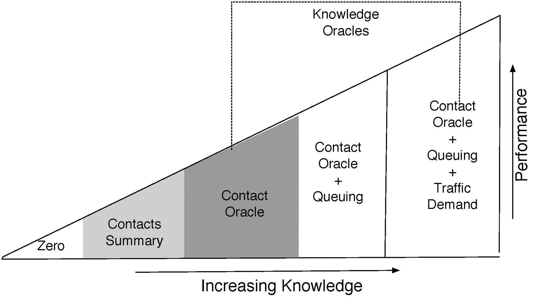
Figure 1. Conceptual performance vs knowledge [16].
As already stated, we can also find several other opportunistic network routing protocols that are based on some type of utility function [10]. Such mechanisms assume that nodes in an opportunistic network tend to visit some locations more often than others, and that node pairs that have had repeated contacts in the past are more likely to have contacts in the future. A probabilistic metric called delivery probability P(A, B), estimates the probability that node A will be able to deliver a message to node B. Additionally, we can find other examples where geographical location and time is also considered part of the history taking advantage of spatial and temporal factors in routing [10,11]. Whatever may be the metric of history, most of these routing protocols work on the realistic premise that node mobility is not truly random.
One of the issues with history gathering is to define the granularity as well as the timespan. Opportunistic networks consist mostly of mobile phones or other portable devices. Several methods have therefore been proposed to summarize the history in such a way that it is does not pose a burden on computational and storage capabilities of the device. Moreover, it is argued that better prediction can be obtained by recent history. Lindgren et al. [12] uses an aging factor associated with probabilistic computations where old values are weighted less than the new ones. Other examples like [13] use a mechanism similar to the sliding window to discard the “obsolete” history. Wang [14] has argued in favor of using the most significant r history readings where significance can be defined on a case-to-case basis. We can also find examples where Kalman filters have been used to reduce the noise (irrelevant history) to assure better prediction [15].
We can find several examples in the past that utilize maximal-flow to improve data dissemination in wireless networks. [16] has presented a theoretically-optimum max-flow routing algorithm that makes EH-WSNs able to transparently adapt to time-varying environmental power conditions during their normal operation. Efficiency of smart antennas can be analyzed in interference prone environments using max-flow [17]. In the case of wireless ad-hoc networks, max-flow can also be used to maximize the traffic flow utility over time while, minimizing the total power or maximizing the time to network partition [18]. Moreover, wireless network access points can deploy intelligent bandwidth allocation policy by jointly distributing the resources for those clients that have overlapping connectivity [19]
3. Why Max-Flow?
Typically, network analysis requires finding a maximal-flow solution to identify bottlenecks when there are capacity constraints on the arcs. The maximum flow problem is structured on a network, however, the arc capacities or upper bounds, are the only relevant parameters. Given a graph where one vertex is considered a source and another is the sink, some object then flows along the edges of the graph from the source to the sink. Each edge along the path is given a maximum capacity that can be transported along that route. The maximum capacity can vary from edge to edge, in which case the remainder must either flow along another edge towards the sink or remain at the current vertex for the edge to clear or to be reduced. Thus, the goal of the maximum flow problem is to determine the maximum amount of throughput in the graph from a source to the sink. Readers interested in background and theoretical proofs of problems related to max-flow may consult [20].
A. Adaption for Opportunistic Networks
One may think of several ways to adapt the maximum flow problem for opportunistic networks. The idea here is to obtain maximum traffic that can flow in an opportunistic network among random source and destination pairs. We have used the contact oracle [7] to obtain the maximum flow between two nodes in the network because maximum flow solution can only be obtained, if we have the knowledge about the whole network. Since the contact oracle can predict the timings of future contacts, the contact oracle max-flow solution will give us the maximum volume transferrable between these selected source and destination (src, dst) pairs. As the contact oracle can deliver the exact contact timings of devices in an opportunistic network, we only need a modified Dijkstra’s algorithm citeJain2004Routing to adapt the computation to obtain maximum flow.
When we think about computing maximum flow with the help of history, we have a choice to obtain the path to destination in two different ways.
1) With contact summary: First, we rely on the contact summary oracle to compute maximum flow. As the contact summary oracle does not posses accurate node contact timings in the network, maximum flow obtained by contact summary oracle is expected to be less than that of the contact oracle. As stated earlier, since several methods are used to limit the size of information provided by the contact summary oracle, we analyze how these methods reduce the traffic flow with the gradual decrease in network information accuracy. The information size can be reduced by aggregating the measures over a defined timespan. Here aggregation refers to the mean values of the contact delays and their durations, thus maximum flow can be computed by extrapolating these aggregated measures. We use these extrapolated measures to forecast for the upcoming timespan.
2) Without contact summary: The second way of computing a path for computing maximum flow is by removing the contact summary oracle. Thus, nodes themselves are responsible for sharing the aggregated delays and other measures among each other. This means that information accuracy is further decreased in contrast to the previous scenario of the contact summary oracle because the information flow through the network is dependent on node mobility. A source can calculate the shortest path using this shared information only if another network node has already shared the measures about the destination with the source.
Thus, we reformulate the max-flow problem in an opportunistic network such that we compute the maximum traffic that can flow between a source and a sink using the mean of the variant capacities of all the paths over a defined timespan. Following are the issues that must be addressed to adapt the maximum flow computation for time varying graphs like opportunistic networks.
1) We must define the terminal condition of maximum flow computation algorithm for opportunistic networks. The maximum flow algorithm does not terminate until the residual capacity of all the paths to the sink is reduced to zero. As we are dealing with time varying graphs, we have limited our analysis by setting up a timespan during which the destination must be accessed directly or indirectly by the source.
2) Another interesting question is how to assure this terminal condition when we do not posses accurate information about the network. As stated earlier, both history variants of maximum flow computation have to predict the paths and these computed paths cannot be guaranteed to be correct. In the case, we have an incorrect path, one of the edges on the incorrect path must be either labeled invalid or disconnected temporarily so that Dijkstra’s algorithm can deliver the next best path. At the same time, the residual capacity of the remainder of this path must be kept intact so that it may still be utilized for further maximum flow computation.
3) Another issue is how strictly a path may be followed when we have inaccurate information. We have used a forwarding strategy that does not follow the computed path in a very strict sense. The flow can be attempted to be propagated to any hop that may bring it closer to destination as shown in Figure 2. Due to this aspect, the labeling of an edge as invalid is further complicated because we cannot identify the most suitable edge to be declared invalid, unless we use another oracle that can tell us which edge was either mistimed or failed to be realized at a particular point in time. This factor introduces more inaccuracy to history based computation of maximum flow and remains an open issue.
4. Simulation Setup
We have considered three different kinds of data sets, all of which have been obtained from CRAWDAD. The

Figure 2. Message propagation: shortcut method.
motivation behind choosing these three traces has been a broad spectrum between dense and sparse networks. Two of the data sets have been synthesized from reality mining project [21] from MIT spans on 16 months, i.e. February 2004 to August 2005 whereas, the third data consist of the SNMP logs for one month from an IBM campus [22].
In the case of the IBM access point trace, SNMP is used to poll access points (AP) every 5 minutes, from July 20, 2002 through August 17, 2002. A total of 1366 devices have been polled over 172 different access points during approximately 4 weeks. We have extracted the traces of 928 devices after discovering the existence of 3 clusters in this network. We then chose the biggest cluster with respect to node count. To turn these samples into continuous data, we assume that the snapshot data remains constant for the next 5 minutes. In the rare cases where this would cause an overlap with another snapshot from another access point, we assume that the transition happens halfway between the two snapshots. We further assume that two nodes that are connected to one access point during the overlapping time period are connected to each other.
The second trace of the MIT cell tower is utilized according to the similar principal that was used for the IBM traces. The only difference is that instead of access points, cell towers are used to gather the contact times of the nodes, thus the resulting network can be characterized as a very dense network due to the high range of the cell tower. Due to several lapses in data gathering mentioned by the creators of the data, only 89 of 100 devices are included in our simulation that visited 32,768 different cell towers.
As the duration span of the MIT reality mining is longer than the IBM trace, we have filtered the MIT data to match the time span of the IBM traces. The span time of the IBM trace is approximately one month whereas for MIT is more than one year, we have chosen one month from cell tower on the basis of the activity, so that the results can be compared. We observed that November 2004 had the maximum activity1 among all the months for which cell tower data has been recorded. Similarly to Bluetooth traces, November 2004 turns out to be the maximum activity month with 81 devices and 12592 distinct cell towers. After this filtering process, IBM access point trace turned out to be a medium sparse network while the MIT cell tower trace turned out to be a dense one.
The sparsest network is obtained from Bluetooth logs (MITBT) where each node scans every five minutes for active Bluetooth neighbors and stored the duration of contact times. Like the MIT trace, we selected one month from Bluetooth traces, i.e. November 2004 showed 1858 Bluetooth nodes suggesting a huge number of undesignated nodes as compared to the designated2 81 nodes that were designated to gather the data. Here it is noteworthy that a few undesignated devices had more connectivity and interaction with the network than the designated nodes.
Simulator:
The motivation behind the simulator is to help us find the delays incurred by flows suffered by networks during the execution of different variations of max-flow algorithms. The output is analyzed on the basis of both the number of src, dst pairs that are connected via routes as well as volume delivered from source to destination. As already mentioned, three different traces have been used that significantly differ in the number of nodes involved, number, frequency, and distinctness of meetings that took place among the participants. We have chosen 100 source and destination pairs, for which we compute the maximum traffic that can flow between them. For access point and cell tower traces, the criterion for source destination selection has been set as the 30th percentile of the devices with respect to online time. For Bluetooth, a more strict limit of the 70th percentile has been set for the selection of source and destination due to the scarcity of the network. The rest of the simulation parameters are summarized in Table 1.
It is imperative to mention that the assumption of two devices being connected to one base-station (access point or cell tower), introduces inaccuracies [23]. On one hand, this is overly optimistic, since two devices attached to the same access point may still be out of range of each other. On the other hand, the data might omit connection opportunities, since two nodes may pass each other at a place where there is no base-station, and, hence, this contact could not be logged. Another issue with these data sets is that the devices are not necessarily co-located with their owner at all times (i.e. they do not always characterize human mobility). Despite these inaccuracies, such traces are a valuable source of data, since they span many months and include thousands of devices. In addition, considering that two nodes connected to the same AP are potentially in contact is not altogether unreasonable, as these devices could indeed communicate through the AP, without using end-to-end connectivity.
A. Analyzed Strategies
Based on the above discussed issues, we have simulated the following three different max-flow strategies for the sake of comparison. However, it is important to mention that in the following experiments, maximum flow computations are not performed simultaneously for all of the source and destination pairs. We compute maximum flow between the first src, dst pair and then we move back in time to select the next pair iteratively. Similarly, we go back in time to compute a new path if the given path provided by the contact summary oracle is not correct. It is also important to mention that our implementations of the below described strategies are of greedy nature with respect to delay (quickest path first). Therefore, it is possible that a better path with longer delay is sacrificed for a quicker path. We have decided for the greedy implementation because one of the terminal conditions of the algorithm is to find all maximum flows that can access the destination within the described timespan. Without this condition the computation overhead is too high.
1) Contact oracle max-flow: This max-flow computation is based on contact oracle [7] where paths provided by oracle iteratively, are consumed as long as there exist no such path to the destination that can deliver the traffic within the desired timespan. The path is computed between 100 pairs of source and destinations with the help of the variant of the Dijkstra’s algorithm. Once the src, dst pair is selected, we follow the mechanism similar to what has been presented in [8] described here in Algorithm 1. This way, max-flow computed between the first pair of src, dst will affect all the next max-flows to be computed later, if they share at least a common edge.
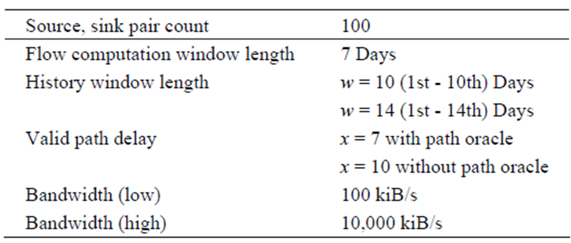
Table 1. Simulation parameters.
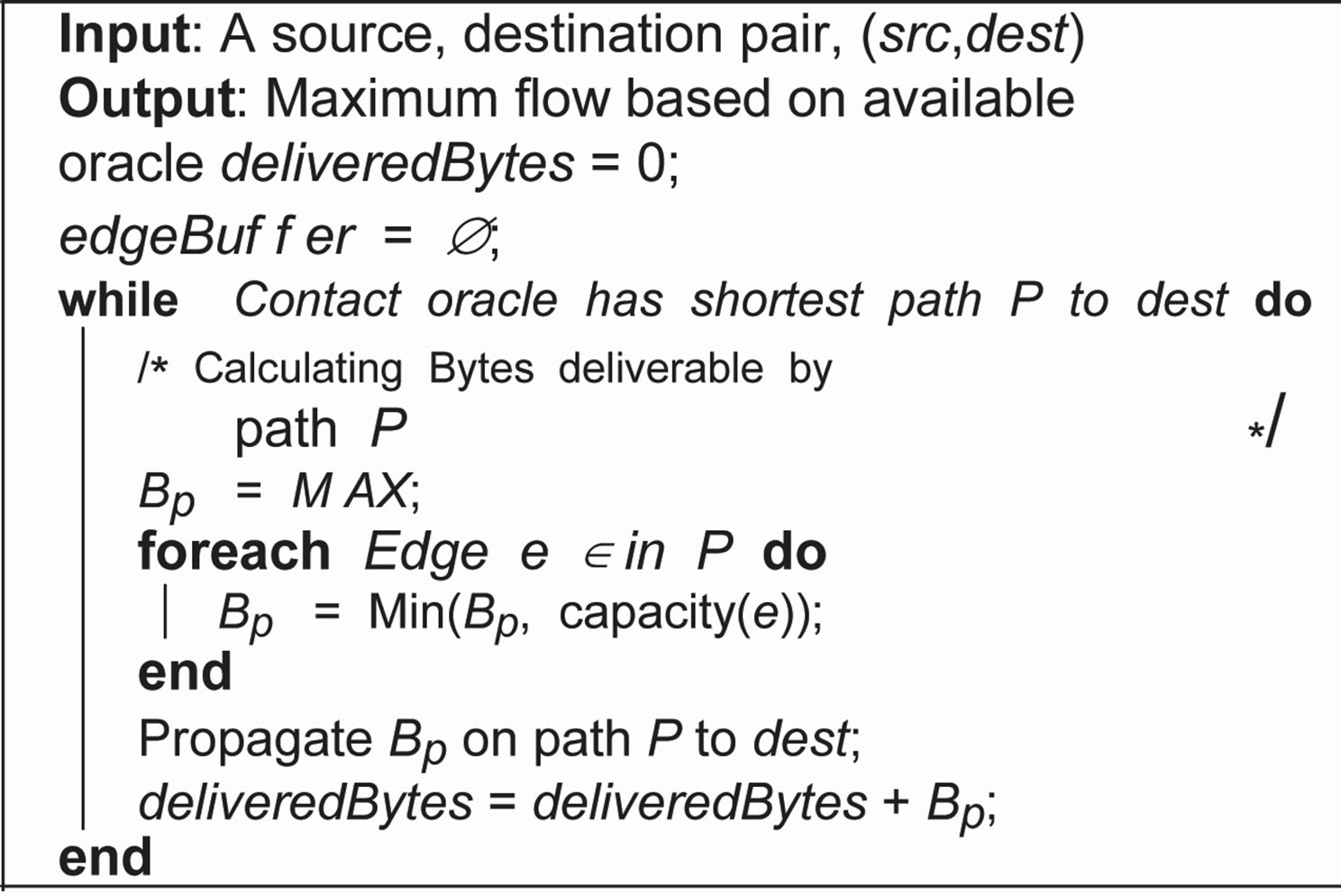
Algorithm 1. Max-flow calculation with help of contact oracle for a given src, dst pair.
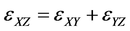
2) History-based max-flow with path oracle: This strategy is a variant of contact summary oracle where we are aware of the delays as well as the mean throughput of the obtained paths. It is imperative to recall that the obtained paths with these measures are used for prediction purpose. These measurements of delays and throughput are accumulated over a defined timespan in the following way. For each encounter between two directly connected nodes X and Y as shown in Figure 3 as direct link, the history information is shared as follows.
a) Node ID of Y if it is a first contact between X and Y.
b) Update or insert mean delay εXY encountered for transmission from X to Y. εXY, includes the time durations, data stay in the local queues as well as inter-hop transmission times.
c) Link throughput. Update mean number of bytes that could be delivered BXY.
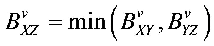
As discussed earlier, contact summary oracle may find a path to the destination but cannot ensure the realization of this path in the network trace. In case, this oracle predicts the path correctly, the probability of correct path throughput prediction is low. Thus, a flow is initiated with the volume that is prescribed by the oracle and this volume is decreased during the propagation if it is realized that the path throughput is less than the volume. This way, different edges on the path may suffer different bandwidth consumptions, which may bring inconsistencies to the results. As there may be several instances of a contact between two devices, we must extrapolate the edges of contact summary oracle proportionally to the frequency of contacts between two devices. These extrapolated edges are consumed in a fashion similar to the mechanism presented in [24] where the aggregated residue capacity on each edge is reduced according to the minimum aggregated capacity of the whole path.
3) History based max-flow without path oracle: This strategy has no access to any oracle. Devices themselves gather and share historical information for a defined timespan. This means we must extend our history gathering method so that direct as well as transitive contacts can be preserved. In addition to the sharing of direct contact history information as described previously, information about indirect contacts is shared in a transitive manner as follows:
For an indirect neighbor or twohop link as shown in Figure 3, device X inserts augmented information in its routing table about the device Z accessible via Ya) Node ID Z if X has no earlier record of Z via Y.

Figure 3. History calculation.
b) Update or insert mean delay from X to Z,
c) Path throughput X, Y, Z,
A source computes maximum flow to the destination, based on these measurements of mutually shared mean delay among the devices. The key difference between with and without path oracle is that the history based max-flow without path oracle does not assure a path, unless the source has been able to obtain the mean delay to the destination from the mutual contacts of the middle hops. Thus, the mobility of a network plays an important role for the dispersion of this information. Theoretically speaking, if nodes in a network move very frequently with the speed of light, we may end up having the same measure as we had in the case of with path oracle variant.
Another question is how to proceed when we have a false prediction. It is possible that the first path is a bad prediction but there may still be available several valid paths that show longer delays. We have to somehow eliminate the current invalid path so that the Algorithm 2 can find the next best predicted path. For the sake of simplicity, we disconnect one edge on the invalid path that has failed to be realized. This means, we disconnect the edge between the last hop successfully taken and the next available hop in the path as shown in Algorithm 3. As our forwarding mechanism does not follow strictly the given path (Figure 2), disconnecting the last hop and next hop may give unexpected results.
B. Amount of History
As discussed in Section 2, a variety of methods can that propose the use of history to predict the behavior of devices can be found in literature. In the light of these examples, we have introduced a window period variable w. This variable represents the timespan over which history is accumulated. The two values used for w are 10 and 14 representing the corresponding timespan in days. To separate the two issues of accuracy loss due to information aggregation from quality of prediction, we have simulated both variations of history based max-flow computation on the same timespan from which history has been computed as well as for 7 following days after the history timespan elapsed. This configuration is represented in Figure 4, where two values of w = 10 and 14 are represented with the corresponding prediction time period.
We have used a threshold of path delay of x = 7 days, i.e. all paths showing longer than 7 mean delays are discarded. The rest of the simulation parameters are summarized in Table 1. It is important to mention here that we have utilized the same history for x = 10 as computed
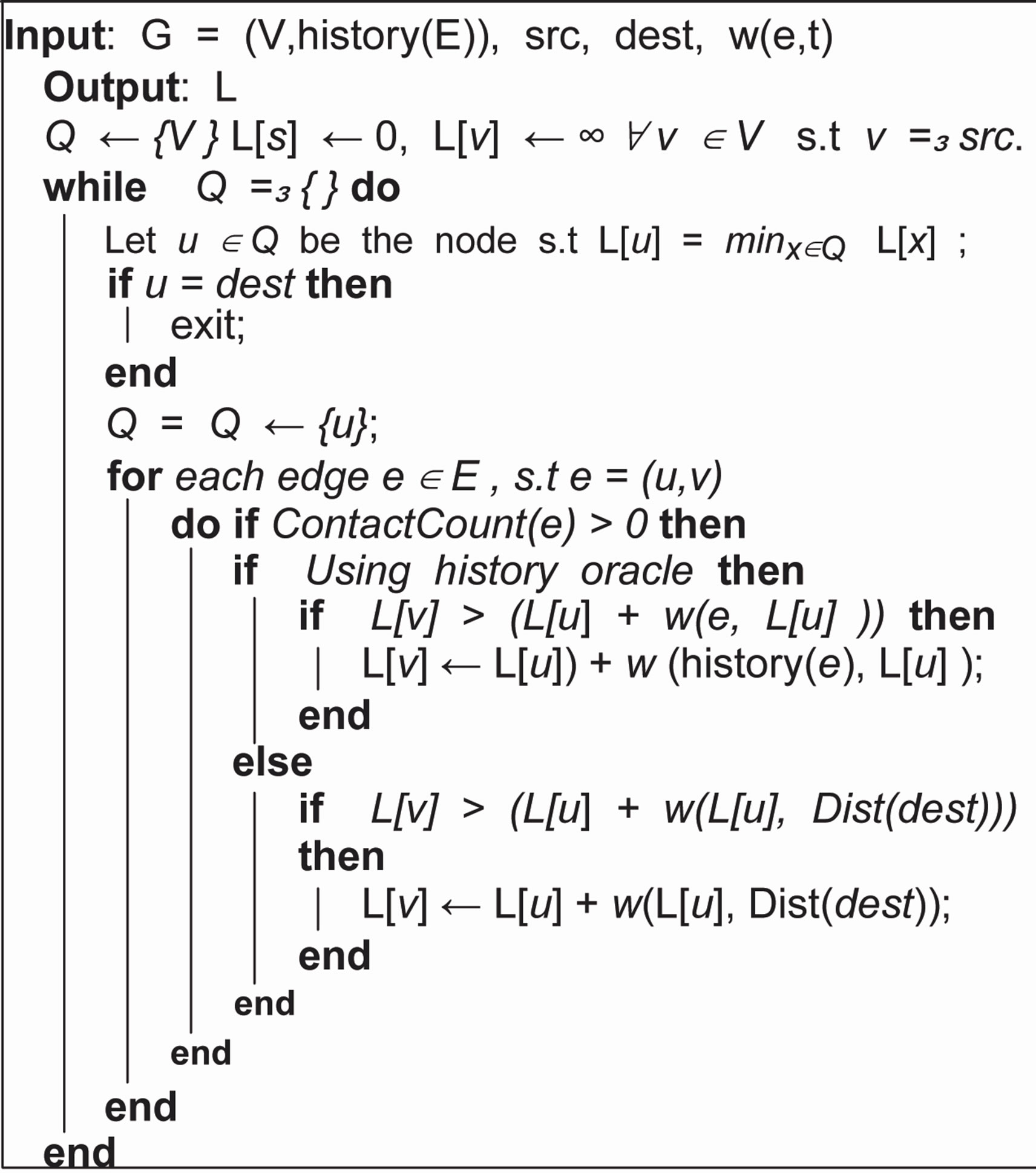
Algorithm 2. Dijkstra’s Algorithm modified to use history costs. src and dst are the source and destination node respectively. The path calculation is performed on the edges provided by history(E), using oracle, we can calculate cost calculated provided by history to every node, however without oracle, we need a destination for which we need to calculate the costs.
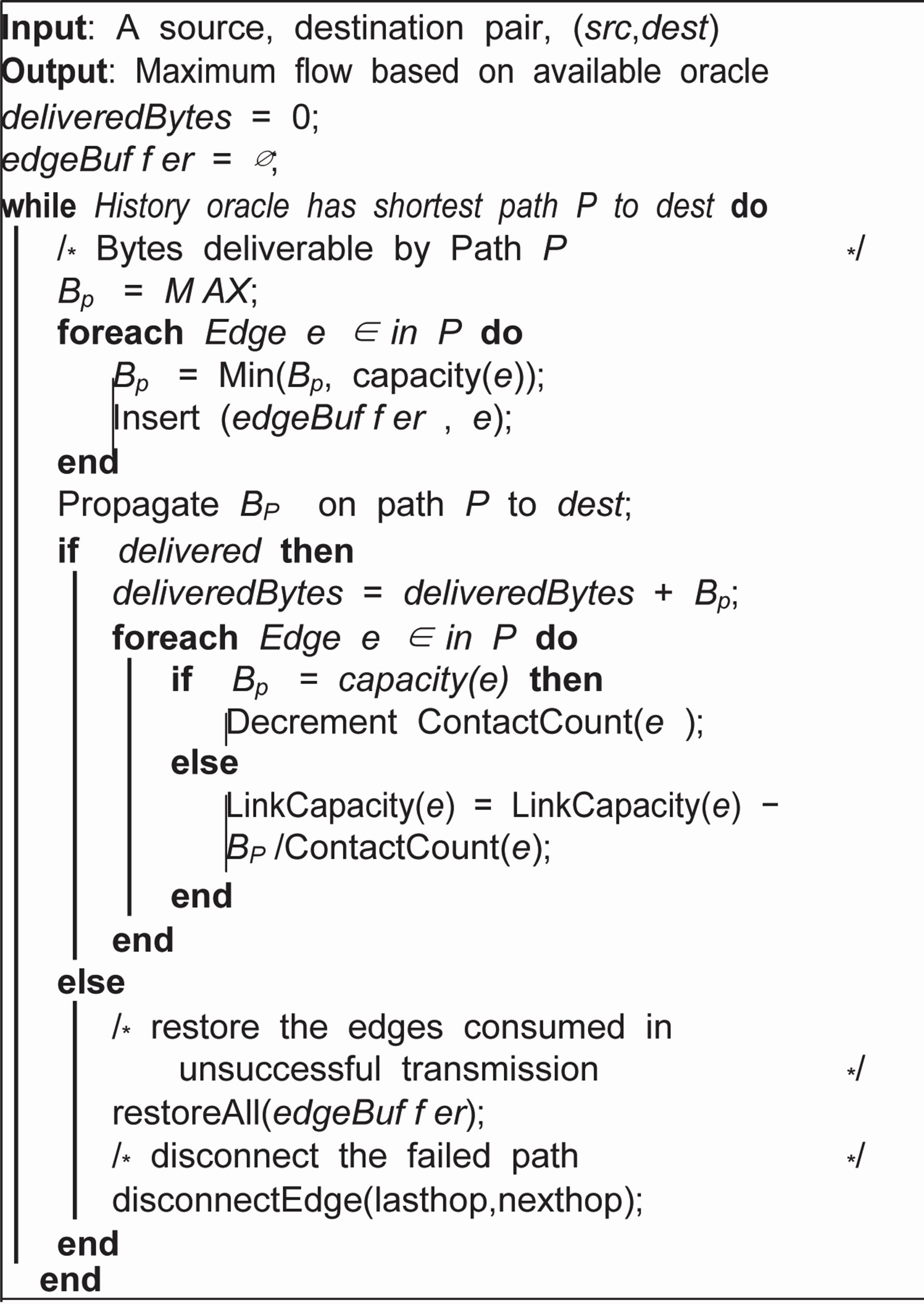
Algorithm 3. Max-flow calculation with help of history oracle for a given src, dst pair.
for opportunistic routing simulations presented in [5]. This aspect resulted in some unexpected outcomes that we are not able to address due to time limitations.
5. Results and Discussion
For the sake of presentation, we have assigned several denotements to our strategies that are presented in Table 2. We have used the suffix-Pred. to represent the predicted max-flow.
This max-flow computation is performed on the timespan of 7 days that starts after history timespan has elapsed shown as unshaded rectangle in Figure 4. Moreover, each denotement is followed by a number that represents the value of history window size, i.e. w.
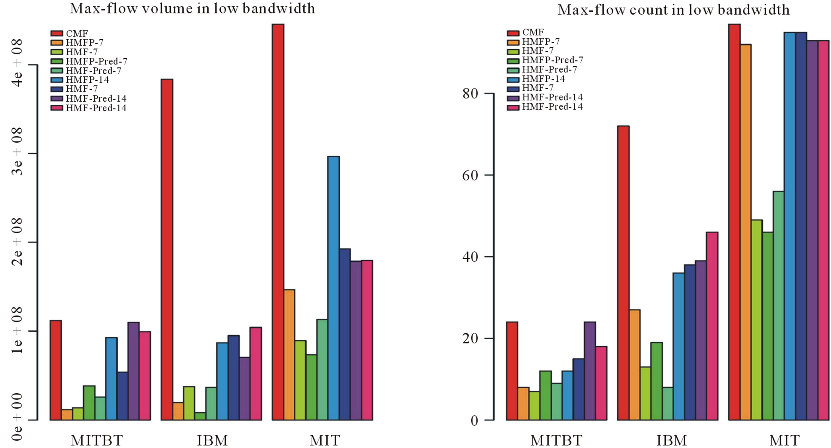
When we look at all the plots in Figures 5 and 6, CMF has delivered the maximum amount of bytes as well as discovered the maximum number of routes between src, dst pairs. The scarcity of the Bluetooth (MITBT) trace is evident here where CMF has discovered a mere 30 routes between src, dst pairs as shown in Figure 5(a). In cell tower (MIT) and access point (IBM) cases, it has discovered routes between 98 and 70 src, dst pairs receptively. We also notice that the difference between high and low bandwidth is visible only in the traffic volume while, the number of src, dst pairs connected via routes is more or less the same.
Another observation that is true for all the 4 figures is that an increase in window size w has a positive effect on almost all of the HMFs variants. Moreover, we see a decrease in both max-flow computations, i.e. volume and count, in almost all cases, when we look at pred. variants. There are a few exceptions to this statement that we will be discussing later.
When we analyze the two sets of results presented here in low bandwidth Figures 5(a) and (b), CMF has delivered maximum bytes as well established contacts between maximum pairs of source and destination in all three traces. When we look at all of the HMFs-7 and HMFP’s-7, we see a drastic decrease in both aspect, i.e. volume and count. We did not expect such a drastic decrease, particularly not in the Bluetooth (MITBT) trace. It is also interesting to observe that HMFP has delivered slightly fewer bytes than HMF but has established one
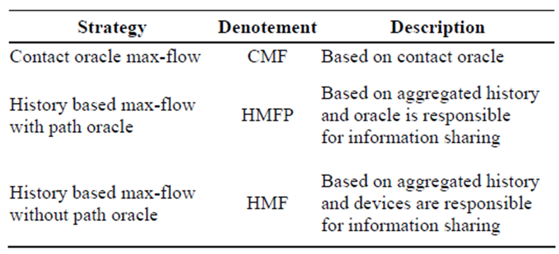
Table 2. Algorithm denotement and description.
more path. Although, HMF is supposed to have more inaccurate information in comparison to HMFP, due to artifacts explained later, it has delivered a few extra bytes in the Bluetooth (MITBT) trace.
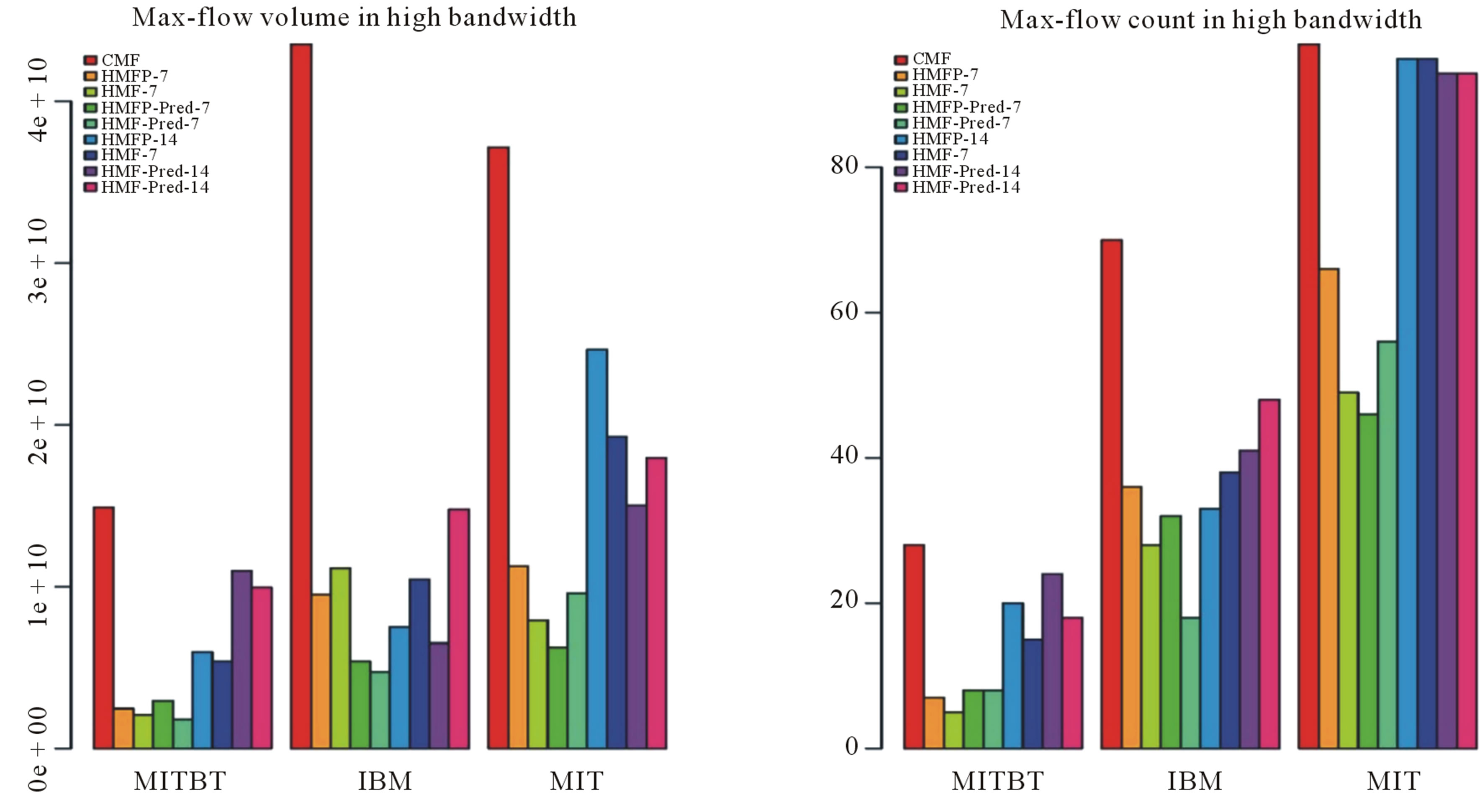
On the contrary, HMFP has delivered more bytes as well as discovered routes between more src, dst pairs in the Bluetooth (MITBT) high scenario (Figure 6(a)). Where HMFP has delivered more data as compared to HMF, the IBM trace has shown the expected behavior as far as volume is concerned (Figure 6(b)). This behavior is consistent for the IBM trace in the high bandwidth scenario however; it is not true for the MIT high bandwidth scenario.
The behavior of the dense MIT network has been as expected because the history window size of 14 has made sure that information about all paths is spread all over the network (Figure 5(a)). All strategies with history window w = 14 have discovered almost all the routes between pairs that CMF has discovered. As far as volume is concerned, (Figure 5(b)), we can see that the decrease in readings, when compared to CMF, is due to information loss to aggregation.
A few inconsistencies that have been observed in the results can be explained with the help of following arguments. As stated earlier, our implementation of the contact summary oracle is greedy with respect to delay (the quickest path first), which means that the utilization of a quicker low throughput path can affect the max-flow computation of a slower high throughput path. Moreover, the artifact of the forwarding scheme depicted in Figure 2 has also resulted in interesting side effects. As discussed, the forwarding scheme combined with the mechanism of removing the invalid path can cause a useful edge to be disconnected. This is due to the fact that we cannot exactly identify the edge on the traversed path that is responsible for the failure without another oracle. Another reason is the variable consumption of edges during volume propagation, in which all history based max-flows may consume less bytes in later edges than the former ones because of the dynamic reduction of flow volume.
When we look at the volumes delivered by CMF in high bandwidth scenario (Figure 6(b)), volume delivered for IBM trace has surpassed all the others, whereas the contact count is higher in the MIT case (Figure 6(a)). Surprisingly, the contact count for HMF is far lower when we compare MIT low and high bandwidth cases. This is because the two HMFs, i.e. low and high, have discovered several routes between same src, dst pairs through different paths because of congestion experienced in low bandwidth. Thus, the larger volume delivered by HMF has caused the history oracle to disconnect
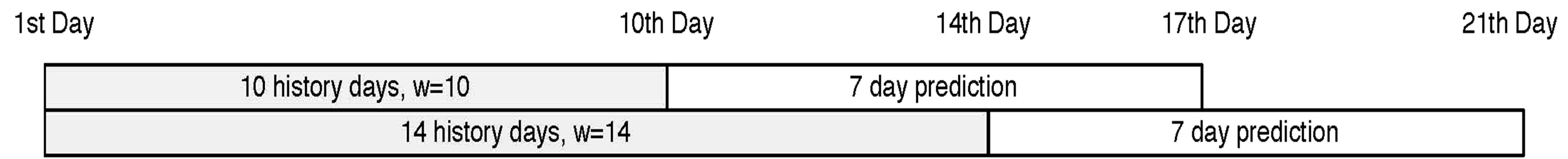
Figure 4. History window and prediction setup configuration.
 (a) (b)
Figure 5. Maximum flow results for low bandwidth scenario (a) src,dest count (b) Volume.
 (a) (b)
Figure 6. Maximum flow results for high bandwidth scenario (a) src,dest count (b) Volume.
the network and the contact count has dropped (Figure 6(b)).
6. Conclusions and Future Work
We have fused concepts from traditional graph theory with the emerging opportunities in mobile wireless environment. Initial results are promising both in terms of admittance and fairness. These max-flow based experiments can be seen as a first attempt to analyze the variance in the behavior of three opportunistic networks while varying variable like bandwidth and window size. We can conclude from these experiments that the variance of all variables may produce counterintuitive results depending on the underlying network. History can bring good quality prediction provided the network devices show regularly consistent behaviors.
In our opinion, it is unlikely for a history computation/gathering mechanism that is universal for every kind of opportunistic network. Thus, history gathering should be an adaptive process in such a way that it can select the statistical methods for acquiring node contact information with respect to the context of underlying network. In a low resource setting with limited mobility, the physical transport of digital data at a frequency of less than once per week should still be acceptable for services that can tolerate such delayed notification of results [25]. Furthermore, the validity of history decays with the passage of time and particularly sparse network suffer this decay in quality. It is also essential to keep the history size in check, although history gathered over longer period does bring some advantages. In our opinion the history window size must be correlated with the mobility of individual devices, i.e. devices with low mobility should have longer window than devices with high mobility.
REFERENCES
- I. Bisio and M. Marchese, “Congestion Aware Routing Strategies for dtn-Based Interplanetary Networks,” Proceedings of the Global Communi-cations Conference, New Orleans, 30 November-4 December 2008, pp. 1-5.
- S. Guo, M. Derakhshani, M. H. Falaki, U. Ismail, R. Luk, E. A. Oliver, S. U. Rahman, A. Seth, M. A. Zaharia and S. Keshav, “Design and Implementation of the Kiosknet System,” Computer Networks, Vol. 55, No. 1, 2011, pp. 264-281. doi:10.1016/j.comnet.2010.08.001
- A. Keranen and J. Ott, “Increasing Reality for dtn Protocol Simulations,” Helsinki University of Technology, Helsinki, 2007.
- J. Burgess, B. Gallagher, D. Jensen and B. Levine, “Maxprop: Routing for Vehicle-Based Disruption-Tolerant Networking,” Proceedings of IEEE Infocom, Barcelona, 23-29 April 2006.
- M. Islam and M. Waldvogel, “Optimizing Message Delivery in Mobile-Opportunistic Networks,” Internet Communications, 2011 Baltic Congress on Future, Riga, 17 February 2011, pp. 134-141. doi:10.1109/BCFIC-RIGA.2011.5733212
- X. Zhuo, Q. Li, W. Gao, G. Cao and Y. Dai, “Contact Duration Aware Data Replication in Delay Tolerant Networks,” IEEE International Conference on Network Protocols, Vancouver, 17-20 October 2011, pp. 236-245.
- S. Jain, K. Fall and R. Patra, “Routing in a Delay Tolerant Network,” Proceedings of SIGCOMM 2004, ACM Press, New York, 2004, pp. 145-158. doi:10.1145/1015467.1015484
- M. A. Islam and M. Waldvogel, “Questioning Flooding as a Routing Benchmark in Opportunistic Networks,” 2011 Baltic Congress on Future Internet Communications, Riga, 17 February 2011, pp. 128-133. doi:10.1109/BCFIC-RIGA.2011.5733215
- L. Lilien, Z. H. Kamal and A. Gupta, “Opportunistic Networks: Chal-Lenges in Specializing the p2p Paradigm,” International Workshop on Database and Expert Systems Applications, Krakow, 4-8 September 2006, pp. 722-726.
- J. Z. J. Liu and H. G. Gong, “Preference Location-Based Routing in Delay Tolerant Networks,” International Journal of Digital Content Technology and its Applications, Vol. 5, No. 4, 2011, pp. 468-474.
- B. Burns, O. Brock and B. N. Levine, “Mv Routing and Capacity Building in Disruption Tolerant Networks,” Proceedings of IEEE Infocom, Miami, 13-17 March 2005.
- A. Lindgren, A. Doria, J. Lindblom and M. Ek, “Networking in the Land of Northern Lights: Two Years of Experiences from dtn System Deployments,” Proceedings of the 2008 ACM Workshop on Wireless Networks and Systems for Developing Regions, ACM, New York, 2008, pp. 1-8. doi:10.1109/TMC.2007.1016
- E. P. C. Jones, L. Li and J. K. Schmidtke, “Practical Routing in Delay-Tolerant Networks,” IEEE Transactions on Mobile Computing, Vol. 6, No. 8, 2007, pp. 943- 959.
- Y. Wang, S. Jain, M. Martonosi and K. Fall, “ErasureCoding Based Routing for Opportunistic Networks,” ACM Workshop on Delay Tolerant Networking, Philadelphia, 26 August 2005.
- P. Costa, C. Mascolo, M. Musolesi and G. P. Picco, “Socially-Aware Routing for Publish-Subscribe in DelayTolerant Mobile Ad Hoc Networks,” IEEE Journal on Selected Areas in Communications, Vol. 26, No. 5, 2008, pp. 748-760. doi:10.1109/JSAC.2008.080602
- A. Seraghiti, S. Delpriori, E. Lattanzi and A. Bogliolo, “Self-Adapting Maxflow Routing Algorithm for wsns: Practical Issues and Simulation-Based Assessment,” Proceedings of the 5th International Conference on Soft Computing as Transdisciplinary Science and Technology, Ser, ACM, New York, 2008, pp. 688-693.
- X. Huang, J. Wang and Y. Fang, “Achieving Maximum Flow in Interference-Aware Wireless Sensor Networks with Smart Antennas,” Ad Hoc Networks, Vol. 5, No. 6, 2007, pp. 885-896. doi:10.1016/j.adhoc.2007.02.003
- T. X. Brown, H. N. Gabow and Q. Zhang, “Maximum Flow-Life Curve for a Wireless Ad Hoc Network,” Proceedings of the 2nd ACM International Symposium on Mobile Ad Hoc Networking & Computing, ACM, New York, 2001, pp. 128-136.
- S. K. Dandapat, B. Mitra, N. Ganguly and R. R. Choudhury, “Fair Bandwidth Allocation in Wireless Network Using Max-Flow,” SIGCOMM—Computer Communication Review, Vol. 41, No. 4, 2010, pp. 22-24.
- R. K. Ahuja, T. L. Magnanti and J. B. Orlin, “Network Flows: Theory, Algorithms, and Applications,” Prentice Hall, Upper Saddle River, 1993.
- N. Eagle and A. S. Pentland, “CRAWDAD Data Set Mit/Reality (v. 2005-07-01),” 2005. http://crawdad.cs.dartmouth.edu/mit/reality
- M. Balazinska and P. Castro, “CRAWDAD Data Set IBM/Watson (v. 2003-02-19),” 2003. http://crawdad.cs.dartmouth.edu/ibm/watson
- A. Chaintreau, P. Hui, J. Crowcroft, C. Diot, R. Gass and J. Scott, “Impact of Human Mobility on the Design of Opportunistic Forwarding Algorithms,” Proceedings of IEEE Infocom, Barcelona, 23-29 April 2006.
- D. R. F. Ford, “Maximal Flow through a Network,” Canadian Jounral of Mathematics, Vol. 8, 1956, pp. 399- 404. doi:10.4153/CJM-1956-045-5
- J. S. S. Syed-Abdul, et al., “Study on the Potential for Delay Tolerant Networks by Health Workers in Low Resource Settings,” Computer Methods and Programs in Biomedicine, 2011, in Press. doi:10.1016/j.cmpb.2011.11.004
NOTES
1Activity is defined as time spent “online” by devices, i.e., being connected to either cell towers or other neighboring devices.
2Nodes running the scanning software are referred to as designated.