Journal of Environmental Protection
Vol.4 No.4(2013), Article ID:30431,11 pages DOI:10.4236/jep.2013.44040
Clusterization of Surface Water Quality and Its Relation to Climate and Land Use/Cover
![]()
1Department of Civil Engineering, Schulich School of Engineering, University of Calgary, Calgary, Canada; 2Department of Geomatics Engineering, Schulich School of Engineering, University of Calgary, Calgary, Canada.
Email: taakbar@ucalgary.ca, tahiraliakbar@yahoo.com, *qhassan@ucalgary.ca, gachari@ucalgary.ca
Copyright © 2013 Tahir Ali Akbar et al. This is an open access article distributed under the Creative Commons Attribution License, which permits unrestricted use, distribution, and reproduction in any medium, provided the original work is properly cited.
Received November 28th, 2012; revised February 26th, 2013; accepted March 25th, 2013
Keywords: Alberta Rivers; Canadian Water Quality Index; Clustering; Geographic Information System; Pattern Recognition; Principal Component Analysis; River Water Quality
ABSTRACT
The quality of surface water is rapidly changing due to climatic variations, natural processes, and anthropogenic activities. The objectives of this study were to classify and analyze the surface water quality of 12 major rivers of Alberta on the basis of 17 parameters during the period of five years (i.e., 2004-2008) using principal component analysis (PCA), total exceedance model and clustering technique. Seven major principal components (PCs) with variability of about 89% were identified. These PCs were the indicators of watershed geology, mineralization and anthropogenic activities related to land use/cover. The seven dominant parameters revealed from the seven PCs were total dissolved solids (TDS), true color (TC), pH, iron (Fe), fecal coliform (FC), dissolved oxygen (DO), and turbidity (TUR). The normalized data of dominant parameters were used to develop a model for obtaining total exceedance. The exceedance values acquired from the total exceedance model were used to determine the patterns for the development of five clusters. The performance of the clusters was compared with the classes obtained in Canadian Water Quality Index (CWQI). Cluster 1, cluster 2, cluster 3, cluster 4 and cluster 5 showed agreements of 85.71%, 83.54%, 90.22%, 80.74%, and 83.40% with their respective CWQI classes on the basis of the data for all rivers during 2004-2008. The water quality was deteriorated in growing season due to snow melting. This methodology could be applied to classify the raw surface water quality, analyze the spatio-temporal trends and study the impacts of the factors affecting the water quality anywhere in the world.
1. Introduction
In general, the quality of waters in rivers and lakes depends on climate, land use, land cover, geographical and anthropogenic factors [1-4]. Climatic factors, such as melting snow over high latitudes and precipitation wash material from the land surface into the water-bodies. Various land use activities (e.g., wood logging, agricultural, mining and urban development) can be potential sources of pollutants, which impact the water quality. Thus, it is important to classify the raw surface water quality and study the spatio-temporal impacts due to anthropogenic activities and climatic factors.
In Alberta, 17 water quality-related parameters are periodically measured for 12 major rivers at 23 fixed sampling sites. These data are then analyzed using the Canadian Water Quality Index (CWQI) system developed by the Canadian Council of Ministers of the Environment (CCME); and represented as an index-value [5]. Despite the robustness and acceptance of CWQI, the data acquisition is labour intensive, time consuming and costly. Thus, it is worthwhile to investigate whether a lesser number of water quality-related parameters would produce similar CWQI-values.
In order to determine data redundancy in any dataset, one of the most commonly used methods is the employment of pattern recognition algorithms [6,7]. Examples of such algorithms are principal component analysis (PCA) and clustering techniques. In PCA, the original set of parameters is transformed into uncorrelated principal components (PCs), which decrease the total variance. Each parameter contributes towards its respective PC and its contribution is determined by the loading values. PCA has been used in many water quality studies, such as 1) determining spatio-temporal changes in the water quality of Jajrood River [8]; 2) comparing water quality of regional sites of Canada for spatial and temporal changes [9]; 3) seasonal and spatial variations for surface water quality of Mid-Black Sea Coast in Turkey [10]; and 4) impact of agricultural activities for Nathan Creek Watershed, British Columbia, Canada [11].
The clustering techniques are used to find structure in data by identifying the groups (clusters) in the data and the objects are grouped on the basis of similarities within a class and dissimilarities among different classes. The similarities and dissimilarities are obtained on the basis of distance measures (e.g., Euclidean, Manhattan, etc.) using various clustering methods [12]. The clustering methods have been widely used in the water quality studies. For example: 1) clustering for chemical classification of water in Salado River [13]; 2) Hierarchical agglomerative cluster analysis for delineating and grouping pollution causing areas [14]; and 3) Fuzzy clustering of water quality parameters for Ulansuhai Lake [15]. In addition to classification of water quality, it is also important to understand the impact of causative factors on the surface water quality of rivers in Alberta. For this purpose geographic information system (GIS) was used as its application was found useful in studying the water quality [16,17]. The objectives of this paper are to: 1) develop clusters for major rivers in Alberta on the basis of monthly water quality data; 2) evaluate the clusters using Canadian Water Quality Index (CWQI) system; 3) apply clusters for spatio-temporal analysis; and 4) study the impact of climatic factor (i.e., snow-melting) and land use activities on the water quality of the rivers.
2. Materials and Methods
2.1. Study Area and Data Requirements
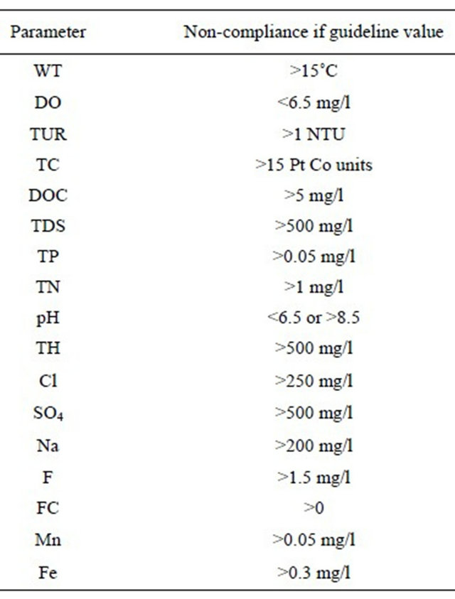
The study area consists of 12 major rivers in Alberta as shown in Figure 1. Alberta is a western province in Canada, which borders the province of British Columbia in west, and Saskatchewan in east. The mean annual temperature in winter varies from −25.1˚C to −9.6˚C and in summer it ranges from 8.7˚C to 18.5˚C. The mean average annual precipitation ranges from 333 mm to 989 mm [18]. The major land use/cover types are needle leaf forests (57.57%), grasses/cereal crops (30.11%) and broad leaf forests (5.25%). The province is dominated by boreal forest in the north and agriculture in the south. At each of the sites, we obtained the monthly values of the 17 water quality-related parameters for the period 2004-2008 from Alberta Environment. These parameters included: chloride (Cl), dissolved organic carbon (DOC), dissolved oxygen (DO), fecal coliforms (FC), fluoride (F), iron (Fe), manganese (Mn), pH, sodium (Na), sulfate (SO4), total dissolved solids (TDS), total hardness (TH), total nitrogen (TN), total phosphorus (TP), true color (TC), turbidity (TUR) and water temperature (WT). There are guideline values for each of these parameters in the context of determining the water quality [19-21]. Those guidelines are summarized in Table 1. In addition,

Figure 1. Location of 23 sampling sites across the twelve major rivers in Alberta. The lengths of rivers are provided in the parenthesis and the arrows show the directions of rivers’ flow.
Table 1. Guidelines for Canadian drinking water quality [19-21].
we also used the maps for land use/cover and snowmelting time period to understand the impact on the surface water quality. Those included: 1) Moderate Resolution Imaging Spectroradiometer (MODIS)-based annual composite land use/cover map at 1 km spatial resolution (MOD12Q1 ver. 004) during 2004 available from National Aeronautics and Space Administration (NASA) [22]; and 2) MODIS-derived snow melting time period map at 500 m spatial resolution during 2008 [23].
2.2. Methods
The methods consisted of three major components, such as: 1) development of clusters; 2) evaluation of clusters; and 3) application of clusters. Brief descriptions of these components are as follows:
2.2.1. Development of Clusters
For the development of clusters, we followed four steps, i.e., 1) normalizing water quality data; 2) obtaining dominant parameters; 3) developing total exceedance model; and 4) identifying the cluster patterns.
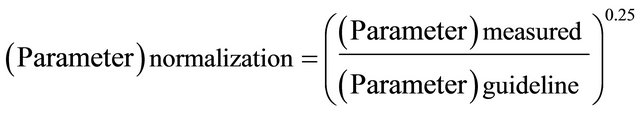
In the first step, the data was normalized for 1) WT, TUR, TC, DOC, TP, TN, TDS, TH, Cl, SO4, pH > 8.5, Na, F, Mn and Fe using Equation (1); and 2) DO and pH < 6.5 using Equation (2).
 (1)
(1)
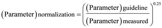 (2)
(2)
In both the above equations (i.e., Equations (1) and (2)) we used the power of a constant number (i.e., 0.25) to reduce the spread between the parameters due to large variations in their measured values. As the guideline was 0 for FC therefore we normalized it by exponention with exponent equal to 0.25.
In the second step, we used PCA to identify the major PCs and obtain the dominant parameters using the normalized data [24]. The numbers of PCs were decided by setting eigenvalue to 0.5 and the loading values of parameters were obtained using varimax normalized rotation [8]. The loading values were divided into three classes (i.e., strong > 0.75, 0.75 > moderate > 0.5 and 0.5 > weak > 0.4). Parameter loading values less than 0.40 were not considered because of their minor significance in the data [25]. From each of the PCs, one of the parameters was selected as the dominant one on the basis of the highest loading-values.
In the third step, the normalized values of dominant parameters were used to develop a model for obtaining the total exceedance for each monitoring day during the period 2004-2008.
In the fourth step, the exceedance values (obtained from the third step) were used to identify the patterns to develop clusters for the classification of surface water quality of the rivers. Seventy percent of the results obtained from the total exceedance model were used to develop the clusters and the remaining thirty percent of the results were used to evaluate them.
2.2.2. Evaluation of Clusters
For quantitative evaluation, the percent cumulative agreements (in the form of deviation) between the clusters and CWQI classes were calculated for: 1) all rivers during the period 2004-2008; and 2) each river during the whole period of 2004-2008. Several equations were used for calculating CWQI (see Table 2 for more details). On the basis of quantitative values (i.e. 0 to 100) calculated using CWQI, the water quality at the sampling sites of rivers was categorized into five classes which are 1) 1: excellent (95 - 100); 2) 2: good (80 - 94); 3) 3: fair (60 - 79); 4) 4: marginal (45 - 59); and 5) 5: poor (0 - 44) [5].
2.2.3. Application of Clusters
The dominant clusters were identified for the growing season (April 1-September 30) and the winter months (Oct 1-March 31) for all the sampling sites during 2004-2008. These dominant clusters were used to under-
Table 2. Equations used for calculation of CWQI and identifying classes using the data of 23 sampling sites for 12 rivers during the period 2004-2008.
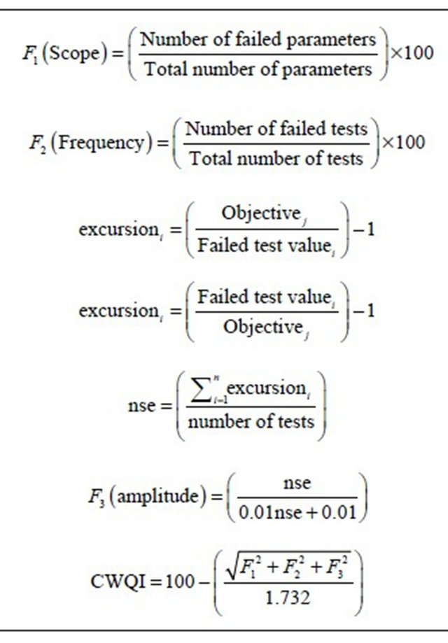
Note: nse: normalized sum of excursion.
stand the: 1) spatio-temporal patterns of the surface water quality of rivers; and 2) impact of land use/cover and snowmelt. To understand the influence of both the factors, all the rivers with their respective sampling sites were overlain in GIS on: MODIS based 1) land use/cover map; and 2) snowmelt time period map.
3. Results and Discussion
3.1. Major Principal Components and the Dominant Water Quality Parameters
PCA led to a set of seven principal components (PCs) using the normalized data during the period 2004-2008. These PCs had eigenvalues greater than 0.5. Individually they captured 31.5%, 20.8%, 12.6%, 9.1%, 6.1%, 5.6%, and 3.4% of the total variance (See Table 3). PC-1 revealed that four ions (i.e., Cl−,  , Na+ and F−) accounted for most of the TDS, which was also related to the variation in TH. Thus it is interpreted as indicator of the watershed geology [26]. TDS was considered as the first dominant parameter due to having highest loading value (i.e., 0.94). PC-2 indicated three correlated parameters (i.e., TC, DOC, and TP). This could be an indi-
Table 3. PCs with loading values for 17 water quality parameters in the five years (2004-2008).
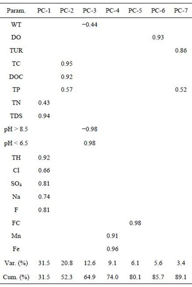
cator of natural and anthropogenic mineralization of water quality [26,27]. In this category, two parameters (i.e. TC and DOC) are strongly positively loaded with TC having the highest loading (i.e., 0.95). TC was considered as the second dominant parameter. PC-3 indicated that pH > 8.5 and pH < 6.5 are strongly loaded with similar magnitudes (i.e., 0.98). WT was weakly negatively loaded in PC-3. In general, temperature increase during the spring season would initiate the process of snow melting, which contributes to the variation of pH in the water. Thus it could be the indicator of anthropogenic activities related to different types of land use/cover [28]. In this component, pH was considered as the third dominant parameter. PC-4 indicated that two parameters (i.e., Mn and Fe) were strongly positively correlated. PC-4 was considered as an indicator of natural mineralization [26]. Fe was considered as the fourth dominant parameter due to its highest loading (i.e., 0.96). PC-5 indicated solely FC as a strongly positively loaded parameter (i.e., 0.98). As FC is related to land cover activities therefore PC-5 could also be the indicator of anthropogenic activities like PC-3. FC was identified as the fifth dominant parameter. PC-6 showed DO as exclusive strongly positively loaded parameter having loading value of 0.93. DO was identified as the sixth dominant parameter. PC-6 was considered as an indicator of natural mineralization like PC-4 [26]. PC-7 indicated TUR as strongly positively loaded and TP as moderately positively loaded parameter. TUR was considered as the seventh dominant parameter due to its highest loading value (i.e., 0.86). The snow melting and precipitation from the different types of land use/cover increase the sediment levels in the surface waters, which increase TUR. In PC-7, both the parameters (i.e., TUR and TP) are related to land cover activities. Like PC-3 and PC-5, it could also be considered as an indicator of anthropogenic activities related to different land cover types [28,29]. Thus, the seven dominant parameters obtained from PCA were: TDS, TC, pH, Fe, FC, DO, and TUR.
3.2. Databases of Clusters and CWQI Classes for Classification of Water Quality
The normalized values of dominant parameters, obtained using Equations (1) and (2), were used to develop a model for obtaining total exceedance as given in Equation (3):
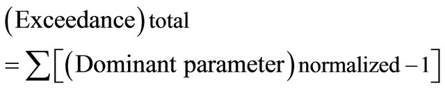 (3)
(3)
Using Equation (3), we calculated the total exceedance values for the normalized data of the dominant parameters during 2004-2008. All of these exceedance values were then used to identify the patterns for the development and evaluation of five clusters. For presentation of cluster patterns in this paper, we used the minimum, maximum and mean exceedance values of dominant parameters as shown in Figure 2. It is obvious that minimum, maximum, and mean increase from cluster 1 towards cluster 5.
We used these clusters to define the water quality of rivers, which could change from cluster 1 towards cluster 5. The water quality deteriorates from cluster 1 to cluster 5. A database of clusters was developed by obtaining the clusters for all the sampling sites of rivers to classify the water quality in each month during 2004-2008. Another database of CWQI classes was also developed for the classification of water quality of rivers during the same time period.
3.3. Comparison of Clusters with CWQI Classes
Figures 3(a) and (b) shows a comparison between % cumulative agreement and deviation for clusters with CWQI classes using the data of all rivers during the period 2004-2008. In the cluster development, the agreements for 0 deviation were 85.71%, 83.54%, 90.22%, 80.74%, and 83.40% for cluster 1, cluster 2, cluster 3, cluster 4 and cluster 5 respectively as shown in Figure 3(a). For the respective five clusters, the agreements for ±1 deviation were 14.29%, 16.46%, 8.83%, 19.26%, and 16.60%. An agreement of 0.95% was observed for ±2 deviation in cluster 3. In the cluster evaluation, the agreements for 0 deviation were 87.50%, 81.82%, 89.51%, 80.64% and 81.63% for cluster 1, cluster 2, cluster 3, cluster 4 and cluster 5 respectively as shown in Figure 3(b). In these five clusters, the agreements for ±1 deviation were 12.50%, 18.18%, 9.09%, 19.36%, and 18.37% respectively. The agreement of 1.40% was found for ±2 deviation in cluster 3. These percentages of agreements showed very close match of clusters with CWQI classes. Table 4 shows the % agreement for the deviations calculated for each river during the period 2004-2008. From Table 4, we found 0 deviation (i.e., 100% agreement) for majority of the rivers for most of the times (i.e., in between 80% - 100% of the cases). In limited number of cases, we observed that the agreement for 0 deviation was between 20% - 73% of the cases for Battle River, Elbow River, Milk River, South Saskatchewan River and Peace River. This difference in agreements from majority of the rivers could be related to the impact of exceedance for parameters other than the dominant once. The quantitative evaluation showed a reasonably strong match between clusters and CWQI classes, which indicates the suitability and usefulness of cluster based classification system for the surface water quality of major rivers of Alberta. The clusters were plotted against CWQI classes for a sampling site of Bow River (i.e., BOR-1) over a period of five years (i.e. 2004-2008) as shown in Figure 4. In this figure, about 90% of observed data showed complete match between clusters and classes whereas only 10% of observed data showed the deviation of ±1. Overall, the patterns of clusters matched quite well with the patterns of CWQI classes as shown in the Figure 4.
3.4. Application of Clusters for Spatio-Temporal Trends
We discussed below the classified water quality for five
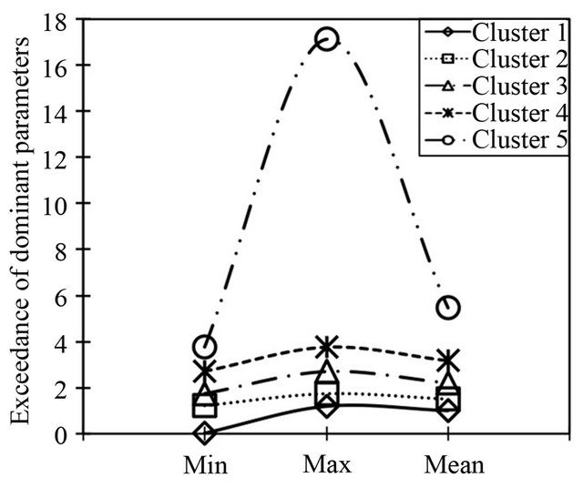
Figure 2. Patterns of five clusters produced from minimum, maximum and mean of the exceedance values of dominant parameters during the period 2004-2008. The exceedance values were calculated using the total exceedance model given in Equation (3).
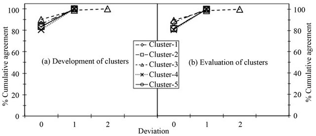
Figure 3. Percentage cumulative agreement between clusters and CWQI classes on the basis of deviations for: (a) Development of clusters; and (b) Evaluation of clusters.
Table 4. Percentage agreement for deviation of clusters on the basis of quantitative evaluation for each river during the period 2004-2008.

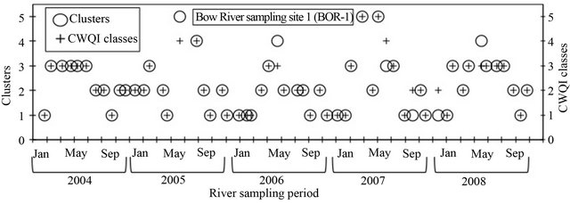
Figure 4. Comparison between clusters and CWQI classes for a sampling site (BOR-1) of the Bow River during the period of 2004-2008.
of the twelve major rivers in Alberta on the basis of clusters. The monthly clusters obtained for these five rivers during the period 2004-2008 are shown in Tables 5-7. An example for studying the spatio-temporal trends from the clusters is presented in Figure 5 for all the sampling sites on the Bow River (see Section 3.4.2). The impacts of land cover (Figure 6(a)) and snow melting (Figure 6(b)) on the water quality of rivers was also discussed in the same sub-sections.
3.4.1. Athabasca River
The dominant cluster for all three sampling sites (AR-1, AR-2 and AR-3) of Athabasca River was cluster 5 during the growing season and it was cluster 3 during the winter season from 2004 to 2008 as shown in Table 5. In 2008, the snowmelt period ranged from 16-May-08 to 24- Jun-08 and 16-May-08 to after 25-Jun-08. This was dominant on the downstream and upstream sides of Athabasca River respectively as shown in Figure 6(b). It
Table 5. Clusters for three sampling sites (AR-1, AR-2, AR-3) of Athabasca River during the period 2004-2008.
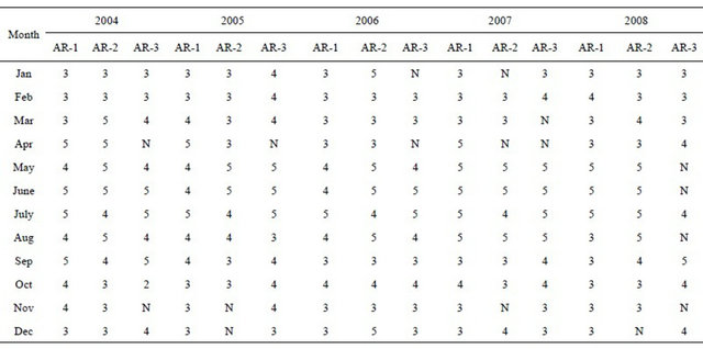
Note: N: no data.
Table 6. Clusters for four sampling sites of Bow River during the period 2004-2008.
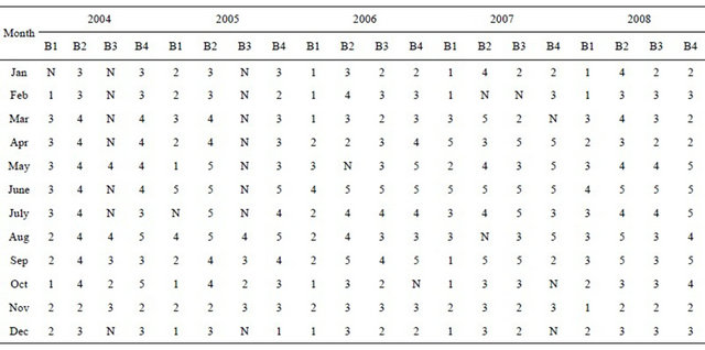
Note: N: no data; B1: BOR-1; B2: BOR-2; B3: BOR-3; B4: BOR-4.
Table 7. Clusters for 1) one sampling site of Milk River; 2) two sampling sites of North Saskatchewan River; and 3) one sampling site of Peace River during the period 2004-2008.
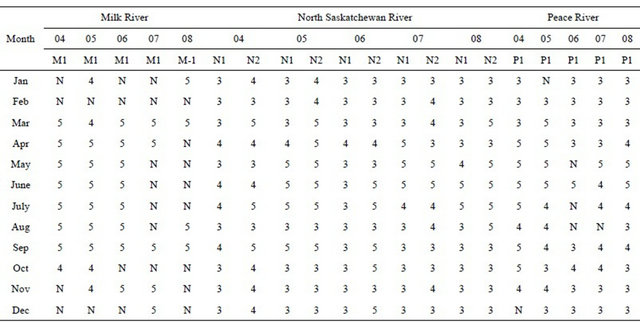
Note: N: no data; M1: MR-1; N1: NSR-1; N2: NSR-2; P1: PR-1.
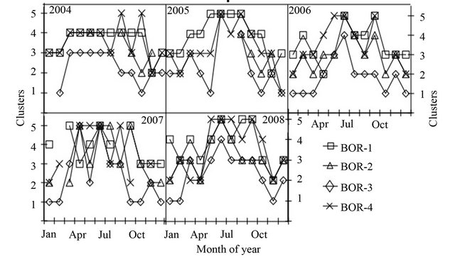
Figure 5. The spatial and temporal trends for the four sampling sites (i.e., BOR-1, BOR-2, BOR-3, and BOR-4) of the Bow River using the clusters during the period of 2004-2008.
indicates that the melting snow is contributing more towards the deterioration in water quality during the growing season as compared to the winter months. The potential sources of deterioration in this river are also the surface runoff from the different land cover types that include needle leaf forests, broad leaf forests and cereal crops/grasses as shown in Figure 6(a). A study done for Athabasca River found that the contamination was associated to land-use related run-off from the forestry and agricultural activities [30].
3.4.2. Bow River
We obtained the dominant clusters from Table 6 for the four sampling sites (BOR-1, BOR-2, BOR-3 and BOR-4) of Bow River during the growing season in the period 2004-2008: 1) BOR-1 belonged to cluster 2 during the period 2005-2006 and cluster 3 in 2004 and 2008; 2) BOR-2 belonged to cluster 4 in 2004 and 2007 and cluster 5 during the periods of 2005-2006 and 2008; 3) BOR-3 fitted in cluster 4 during 2004-2005 and 2008, cluster 3 in 2006 and cluster 5 in 2007; 4) BOR-4 belonged to cluster 4 in 2004, cluster 3 in 2005 and cluster 5 in 2006-2008. From Table 6, it was obvious that during the winter season, the dominant cluster was 1) cluster 1 for BOR-1 in 2004 and 2006-2008; 2) cluster 3 for BOR-2 in 2004-2008; 3) cluster 2 for BOR-3 in the periods of 2006-2007 and cluster 3 in 2008; 4) cluster 3 for BOR-4 in 2004-2007. In 2008, the change in clusters
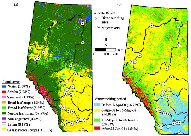
Figure 6. Overlay of the major rivers with their sampling sites on: (a) Land use/cover classes and (b) Snow melting periods.
from winter to growing season for all sampling sites was related to snow melting period. Figure 6(b) indicates that the snow melting period in year 2008 started earlier (i.e., before 5-Apr-08) for BOR-2, BOR-3 and BOR-4 as compared to snow melting period of BOR-1 (i.e., 6-Apr-08 to 15-May-08). The snow melting period could also contribute towards the deterioration of surface quality of Bow River in 2004-2007. The cluster results also revealed that the surface water quality of Bow River in BOR-2, BOR-3 and BOR-4 deteriorated as compared to BOR-1 during the growing season. This was related to the agricultural activities of cereal and broad leaf crops as these three sites are located in adjacent agricultural areas as shown in Figure 6(a). In comparison, BOR-1 is located near a needle leaf forest. Agriculture consumes 90% of the total water usage in South Saskatchewan River Basin and the Bow River is one the major rivers of this basin [28].
3.4.3. Milk River
For the sampling site (MR-1) of Milk River, the dominant cluster was cluster 5 in growing season as well as in winter during the period 2004-2008 as given in Table 7.
The dominant land cover type around Milk River is cereal crops/grasses and the snow melting period around this river was before 5-April-08 as shown in Figures 6(a) and (b) respectively. The deteriorated water quality of Milk River in growing season was because of agricultural activities and surface runoff due to snow melting. The natural mineralization in Milk River due to manganese and iron could be a significant factor for unsatisfactory water quality throughout the year [26].
3.4.4. North Saskatchewan River
Table 7 shows that the dominant cluster for both sampling sites (NSR-1 and NSR-2) of North Saskatchewan River was cluster 3 each year in winter during the period 2004-2008 except 2004 for NSR-2 in which it was cluster 4. During the growing season, the dominant cluster was: 1) cluster 4 in 2004, cluster 5 in 2005 and 2007, and cluster 3 in 2006 and 2008 for NSR-1; 2) cluster 4 in 2004, cluster 5 in 2005-2006 and 2008 and cluster 3 in 2007 for NSR-2. A major portion of North Saskatchewan River along with their sampling sites is dominated by cereal crops/grasses on downstream side of the river and on the upstream side it is covered mostly by needle leaf and broad leaf forests according to the land cover classes shown in Figure 6(a). Cluster 4 and cluster 5 for NSR-1 and NSR-2 in the growing seasons during the period 2004-2008 were due to the agricultural activities. In 2008, the snow melting period was between 6-Apr-08 to 15-May-08; which changed the cluster from 1) cluster 3 in April to cluster 4 in May for NSR-1; and 2) cluster 3 in April to cluster 5 in May for NSR-2 as shown in Figure 6(b). The variation of clusters in different months during the period 2004-2008 was related to snow melting. The potential sources of contamination for the North Saskatchewan River could be the pollutants carried by snowmelt from the activities related to agriculture and forestry [31].
3.4.5. Peace River
The dominant cluster was cluster 3 for PR-1 in winter season during the period 2004-2008 as obvious from Table 7. From this table, we also observed that during the growing seasons, the dominant cluster for PR-1 was: 1) cluster 5 in 2004-2005; 2) cluster 3 in 2006; and 3) cluster 4 in 2007-2008. Most of Peace River is in the snow melting period of 6-Apr-08 to 15-May-08 as shown in Figure 6(b); due to which it was observed that PR-1 had cluster 3 from January to March and cluster 4 in April and cluster 5 from May to June during the year 2008. The reason for the variation in the cluster during the winter and growing seasons for the period 2004-2007 is related to snowmelt period as it was observed for the year 2008. The land cover map (Figure 6(a)) shows that the upstream of Peace River and the area surrounded by the sampling site (PR-1) have cereal crops/grasses whereas the downstream of Peace River is dominated by needle leaf forests. The potential sources of contamination were runoff due to the forests and the agricultural activities [30].
4. Conclusions
In this paper, we classified and analyzed the surface water quality for 12 major rivers in Alberta using the data of 17 parameters for 23 sampling sites during 2004-2008. For classifying the water quality, the clusters were developed and evaluated using CWQI. We developed the normalization models on the basis of Canadian water quality guidelines. The normalized data was then used for PCA to obtain the PCs and identify the dominant parameters. The dominant parameters were used to develop the total exceedance model. The exceedance values of dominant parameters were used to generate the clusters on the basis of identified patterns. The clusters were applied for spatio-temporal analysis. From PCA, we found that PC-1 was indicator of watershed geology. PC-2, PC-4, and PC-6 were indicators of natural and anthropogenic mineralization. PC-3, PC-5 and PC-7 were indicators of activities related to land use/cover. The clusters for all the rivers showed a very strong relationship with CWQI classes. From the cluster analysis, mostly higher (worse condition) cluster number (i.e. 4, 5) were observed for majority of the rivers in the growing seasons as compared to the lower cluster numbers (i.e. 1, 2, 3) in the winters. These would be related to the fact that the snow melting would potentially deteriorate the water quality due to anthropogenic activities from different land use/cover as interpreted in PC-3, PC-5 and PC-7. The agricultural activities were also responsible for deteriorating the water quality of rivers during the growing seasons. We observed the most deteriorated water quality for Battle River and Milk River. The methodology of this study was useful in: 1) grouping a large set of parameters into smaller set of meaningful PCs; 2) interpreting each PC for some natural or anthropogenic activity; 3) identifying the dominant parameters; 4) classifying the large water bodies into clusters; 5) identifying the patterns of clusters; 6) performing the spatial analysis; 7) obtaining the temporal trends; and 8) identifying the potential contamination sources. We suggest applying this method for monitoring, classifying and analyzing the surface water quality in an economical, efficient and user-friendly manner.
5. Acknowledgements
We greatly acknowledge funding in the form of “Postgraduate Scholarship at Doctoral level (PGS-D3)” from Natural Sciences and Engineering Research Council of Canada (NSERC) to Tahir Ali Akbar. The financial assistance from the University of Calgary is gratefully acknowledged. We also acknowledge Alberta Environment, NASA, and N. Sekhon for providing water quality data, MODIS-based annual composite land use/cover map, and MODIS-derived snow melting map respectively.
REFERENCES
- S. Mahapatra and S. Mitra, “Managing Land and Water under Changing Climatic Conditions in India: A Critical Perspective,” Journal of Environmental Protection, Vol. 3, No. 9, 2012, pp. 1054-1062. doi:10.4236/jep.2012.39123
- A. García-Reiriz, J. Magallanes, M. Vracko, J. Zupan, S. Reich and D. Cicerone, “Multivariate Chemometric Analysis of a Polluted River of a Megalopolis,” Journal of Environmental Protection, Vol. 2, No. 7, 2011, pp. 903- 914. doi:10.4236/jep.2011.27103
- B. Toth, D. R. Corkal, D. Sauchyn, G. V. D. Kamp and E. Pietroniro, “The Natural Characteristics of the South Saskatchewan River Basin: Climate, Geography and Hydrology,” Prairie Forum, Vol. 34, No. 1, 2009, pp. 95- 127.
- Z. Zhu, K. Broersma and A. Mazumder, “Impacts of Land Use, Fertilizer and Manure Application on the Stream Nutrient Loadings in the Salmon River Watershed, South-Central British Columbia, Canada,” Journal of Environmental Protection, Vol. 3 No. 8, 2012, pp. 809-822. doi:10.4236/jep.2012.328096
- Canadian Council of Ministers of the Environment (CCME), “Canadian Water Quality Index 1.0 Technical Report and User’s Manual,” Canadian Environmental Quality Guidelines Water Quality Index Technical Subcommittee, Gatineau, 2001.
- I. Eneji, A. Onuche and R. Sha’Ato, “Spatial and Temporal Variation in Water Quality of River Benue, Nigeria,” Journal of Environmental Protection, Vol. 3, No. 8, 2012, pp. 915-921. doi:10.4236/jep.2012.328106
- Y. Singh and M. Kumar, “Interpretation of Water Quality Parameters for Villages of Sanganer Tehsil, by Using Multivariate Statistical Analysis,” Journal of Water Resource and Protection, Vol. 2, No. 10, 2010, pp. 860-863.
- H. Razmkhah, A. Abrishamchi and A. Torkian, “Evaluation of Spatial and Temporal Variation in Water Quality by Pattern Recognition Techniques: A Case Study on Jajrood River (Tehran, Iran),” Journal of Environmental Management, Vol. 91, No. 4, 2010, pp. 852-860. doi:10.1016/j.jenvman.2009.11.001
- S. de Rosemond, D. C. Duro and M. Dubé, “Comparative Analysis of Regional Water Quality in Canada Using the Water Quality Index,” Environmental Monitoring and Assessment, Vol. 156, No. 1-4, 2009, pp. 223-240. doi:10.1007/s10661-008-0480-6
- F. Akbal, L. Gürel, T. Bahadır, İ. Gürel, G. Bakan and H. Büyükgüngör, “Multivariate Statistical Techniques for the Assessment of Surface Water Quality at the Mid-Black Sea Coast of Turkey,” Water, Air, & Soil Pollution, Vol. 216, No. 1-4, 2011, pp. 21-37. doi:10.1007/s11270-010-0511-0
- V. Furtula, H. Osachoff, G. Derksen, H. Juahir, A. Colodey and P. Chambers, “Inorganic Nitrogen, Sterols and Bacterial Source Tracking as Tools to Characterize Water Quality and Possible Contamination Sources in Surface Water,” Water Research, Vol. 46, No. 4, 2012, pp. 1079-1092. doi:10.1016/j.watres.2011.12.002
- L. Kaufman and P. J. Rousseeuw, “Finding Groups in Data—An Introduction to Cluster Analysis,” John Wiley & Sons Inc., New York, 1990. doi:10.1002/9780470316801
- N. A. Gabellone, L. Solari, M. Claps and N. Neschuk, “Chemical Classification of the Water in a Lowland River Basin (Salado River, Buenos Aires, Argentina) Affected by Hydraulic Modifications,” Environmental Geology, Vol. 53, No. 6, 2008, pp. 1353-1363. doi:10.1007/s00254-007-0745-3
- P. K. Srivastava, S. Mukherjee, M. Gupta and S. K. Singh, “Characterizing Monsoonal Variation on Water Quality Index of River Mahi in India Using Geographical Information System,” Water Quality, Exposure, and Health, Vol. 2, No. 3-4, 2011, pp. 193-203.
- C. Ren, C. Li, K. Jia, S. Zhang, W. Li and Y. Cao, “Water Quality Assessment for Ulansuhai Lake Using Fuzzy Clustering and Pattern Recognition,” Chinese Journal of Oceanology and Limnology, Vol. 26, No. 3, 2008, pp. 339- 344. doi:10.1007/s00343-008-0339-2
- T. A. Akbar and R. A. Akbar, “Pesticide Health Risk Mapping and Sensitivity Analysis of Parameters in Groundwater Vulnerability Assessment,” Clean—Soil, Air, Water, 2013. doi:10.1002/clen.201200232
- T. A. Akbar and H. Lin, “GIS based ArcPRZM-3 Model for Bentazon Leaching towards Groundwater,” Journal of Environmental Sciences, Vol. 22, No. 12, 2010, pp. 1854- 1859. doi:10.1016/S1001-0742(09)60331-4
- D. J. Downing and W. W. Pettapiece, “Natural Regions and Subregions of Alberta, Natural Regions Committee,” Government of Alberta, Alberta, 2006.
- Health Canada, “Guidelines for Canadian Drinking Water Quality,” Federal-Provincial-Territorial Committee on Drinking Water of the Federal-Provincial-Territorial Committee on Health and the Environment, 2010.
- Ontario Drinking Water Standards, “Technical Support Document for Ontario Drinking Water Standards, Objectives and Guidelines,” Ministry of the Environment, Drinking Water Ontario, Government of Ontario, Toronto, 2006.
- Alberta Environment and Sustainable Resource Development, “Alberta River Water Quality Index: Objectives, Water Data,” Environment and Water, Government of Alberta, Ottawa, 2011.
- National Aeronautics and Space Administration (NASA), “MODIS/Terra Land Cover Type Yearly L3 Global 1km SIN Grid V004, Land Cover Product, MOD12Q1, LP DAAC User Services,” US Geological Survey, Center for Earth Resources Observation and Science (EROS), Sioux Falls, 2004.
- N. S. Sekhon, Q. K. Hassan and R. W. Sleep, “Evaluating Potential of MODIS-Based Indices in Determining “Snow Gone,” Stage Over Forest-Dominant Regions,” Remote Sensing, Vol. 2, No. 5, 2010, pp. 1348-1363. doi:10.3390/rs2051348
- T. A. Akbar, Q. K. Hassan and G. Achari, “A Methodology for Clustering Lakes in Alberta on the Basis of Water Quality Parameters,” Clean—Soil, Air, Water, Vol. 39, No. 10, 2011, pp. 916-924. doi:10.1002/clen.201100050
- U. C. Panda, S. K. Sundaray, P. Rath, B. B. Nayak and D. Bhatta, “Application of Factor and Cluster Analysis for Characterization of River and Estuarine Water Systems— A Case Study: Mahanadi River (India),” Journal of Hydrology, Vol. 331, No. 3-4, 2006, pp. 434-445. doi:10.1016/j.jhydrol.2006.05.029
- A.-M. Anderson, “River Water Quality of Battle River,” Water Sciences Branch, Water Management Division, Natural Resources Service, Alberta Environment, Edmonton, 1999.
- B. B. Wolfe, T. L. Karst-Riddoch, R. I. Hall, T. W. D. Edwards, M. C. English, R. Palmini, S. McGowan, P. R. Leavitt and S. R. Vardy, “Classification of Hydrological Regimes of Northern Floodplain Basins (Peace-Athabasca Delta, Canada) from Analysis of Stable Isotopes (18O, 2H) and Water Chemistry,” Hydrological Processes, Vol. 21, No. 2, 2007, pp. 151-168. doi:10.1002/hyp.6229
- J. Bruneau, D. R. Corkal, E. Pietroniro, B. Toth and G. V. D. Kamp, “Human Activities and Water Use in the South Saskatchewan River Basin,” Prairie Forum, Vol. 34, No. 1, 2009, pp. 129-152.
- A. Sosiak and J. Dixon, “Impacts on Water Quality in the Upper Elbow River,” Water Science and Technology, Vol. 53, No. 10, 2006, pp. 309-316. doi:10.2166/wst.2006.326
- F. J. Wrona, J. Carey, B. Brownlee and E. McCauley, “Contaminant Sources, Distribution and Fate in the Athabasca, Peace and Slave River Basins, Canada,” Journal of Aquatic Ecosystem Stress and Recovery, Vol. 8, No. 1, 2000, pp. 39-51. doi:10.1023/A:1011487605757
- P. Mitchell, “Water quality of the North Saskatchewan River in Alberta,” Surface Water Assessment Branch, Technical Services and Monitoring Division, Alberta Environmental Protection, Edmonton, 1994.
NOTES
*Corresponding author.