Journal of Environmental Protection
Vol. 3 No. 9A (2012) , Article ID: 22951 , 4 pages DOI:10.4236/jep.2012.329132
An Integrated Agent-Based Framework for Assessing Air Pollution Impacts
![]()
CSIRO Centre for Complex Systems Science, CSIRO Marine and Atmospheric Research, Commonwealth Scientific and Industrial Research Organisation, Canberra, Australia.
Email: *david.newth@csiro.au
Received June 18th, 2012; revised July 15th, 2012; accepted August 9th, 2012
Keywords: Agent-Based Models; Air Quality; Air Pollution
ABSTRACT
Air pollution has considerable impact on human health and the wellbeing. Thus many regions of the world have established air pollution standards to ensure a minimum level of air quality. Precise assessment of the health and socio-economic impacts of air pollution is, however, a complex task; indeed, methods based within an epidemiological tradition generally underestimate human risk of exposure to polluted air. In this study, we introduce an agent-based modeling approach to ascertaining the impact of changes in particulate matter (PM10) on mortality and frequency of hospital visits in the greater metropolitan region of Sydney, Australia. Our modeling approach simulates human movement and behavioral patterns in order to obtain an accurate estimate of individual exposure to a pollutant. Results of our analysis indicate that a 50% reduction in PM10 levels (relative to the baseline) could considerably lower mortality, respiratory hospital admissions and emergency room visits leading to reduced pressure on health care sector costs and placing lower stress on emergency medical facilities. Our analysis also highlights the continued need to avoid significant increases in air pollution in Sydney so that associated health impacts, including health care costs, do not increase.
1. Introduction
Air pollution is a persistent public health concern in major cities throughout Australia and around the world. Those individuals who are particularly susceptible to the deleterious effects of air pollution include the very young, the elderly and those with pre-existing health conditions. Thus the health impacts associated with air pollution are substantial. For example, in 2005 air pollution-related health costs in Sydney were estimated to be AUD $4.7 billion [1]. In major Australian cities, environmental protection and pollution control measures have been established in recognition of the direct and indirect health and economic consequences that air pollutants such as ozone, nitrous oxide and particulate matter (PM10) have on urban communities.
In Australia, environmental information systems deliver information on the air quality in capital cities and their regional areas. In this study, we combine the output from air-quality information systems with an agent-based demographic model as an integrated approach to assess the health, social, and economic impacts of air pollutants, particularly PM10. Traditional epidemiological studies of urban air pollution generally assume that each individual within a city has the same exposure to a pollutant, and this remains static during the analysis. Our approach differs from traditional epidemiological studies through the use of a variant of the agent-based model EpiCast [2,3]. Our variant, called Epidemiological Forecasting of Air Pollution Impacts (EpiCast-API) simulates human movement and behavioral patterns in order to gain a more accurate estimate of individual exposure to a pollutant. By doing this, we are able to more realistically estimate population-level outcomes such as health, social, and economic impacts.
In the following section, we describe EpiCast-API and its overall integrated model framework; the dose-response functions, that link individual exposure to PM10 to particular health outcomes; and how we coupled them to the air-quality information system, TAPM (The Air Pollution Model) [4-6]. Next, we demonstrate how EpiCastAPI can be used to assess the impacts of changes in air pollution levels, focusing on Sydney, the capital of New South Wales in Australia. We examine the impacts of each illustrative scenario in terms of changes in public health outcomes, such as changes in mortality, emergency room visits, and hospital admissions due to respiratory distress. Finally we discuss the simulation results from scenario analysis including their wider implications.
2. Epidemiological Forecasting of Air Pollution Impacts
The overall integrated model framework used in this study (Figure 1) consists of three major components: 1) an air pollution module, based on TAPM; 2) a population module, based on EpiCast, that uses a) a spatially resolved synthetic population of Sydney (based on census data), b) information on human movement, travel, and time usage patterns, and c) a pollutant dose response function; and 3) an analysis module, which focuses on the analysis and visualization of health, social, and economic impacts. We will describe the first two modules here, and the output from the third module is presented in Section 3, as part of the simulations and results.
2.1. Air Pollution Module
The air pollution module is responsible for generating spatially resolved pollution fields with the use of TAPM [4-6]. TAPM is a three-dimensional prognostic model that simulates atmospheric behavior and the dispersion of emissions to predict ground-level concentrations of pollutants. TAPM produces spatially resolved predictions of the concentrations of non-reactive pollutants, primary (PM10) and secondary (PM2.5) particulate matter, sulfur dioxide, and the reactive pollutants, such as nitrogen dioxide and ozone. For this study, we use TAPM with a resolution of 1.5 km2 and divide the Sydney study area into the 3712 sites shown in Figure 2. For each grid cell, TAPM provides daily information on maximum, minimum, and average daily temperature; average and maximum specific and relative humidity; average and maximum ozone concentrations; average and maximum nitrogen dioxide concentrations; and average PM10 and PM2.5 concentrations. While the focus of this study is on the effects of PM10, the overall framework can be expanded to include any of the available pollutants. To illustrate the output from TAPM, Figure 3 shows the daily average PM10 concentrations for the Sydney study area over three successive days.
2.2. Population Module
The population module of our framework is based on the EpiCast agent-based model [2,3]. It has three basic components: 1) a spatially resolved population; 2) human movement and time usage; and 3) pollution dose-response functions, as described below.
2.2.1. Spatially Resolved Synthetic Population
As the basis for our synthetic population, we use a discrete-time, stochastic simulation model of the greater Sydney metropolitan region. The synthetic population,
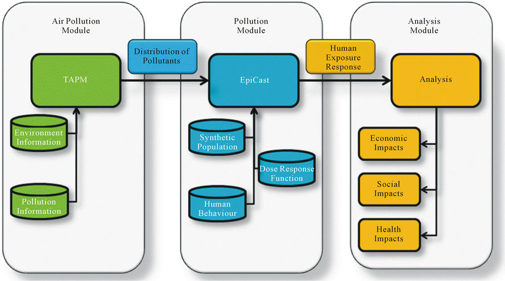
Figure 1. Integrated agent-based framework for assessing air pollution impacts. The three major components: 1) an air pollution module, based on TAPM; 2) a population module, based on EpiCast; and 3) an analysis module, which focuses on the analysis and visualization of health, social, and economic impacts.
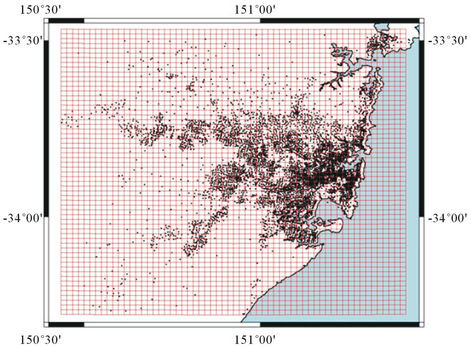
Figure 2. Spatial distribution of census collection districts in the Sydney greater metropolitan region. The dots represent the census districts.
for this region is just over 3.8 million individuals distributed among 65,334 census districts, and calibrated against the 2006 Australian census data [7]. Figure 2 illustrates the spatial distribution of census districts over this region, and shows how these census districts, places of work, schools and other activities are mapped into TAPM cells. As described below, the individuals within each census district are exposed to the level of pollution in the corresponding TAPM cell.
The model population was stochastically generated to match census district distributions of gender, age, family structure, household size, and employment status. Each individual in the population belonged to one of five age groups: preschool-aged children (0 - 4 years), schoolaged children (5 - 19 years), young adults (20 - 29 years), middle-aged adults (30 - 64 years), and older adults (65+ years). The individuals are then arranged into family structures: singles, couples with children, couples without children, and single-parent families. Family sizes range in size from 1 to 7+ members. Families are then arranged into households. Households represent dwellings (e.g., free-standing homes, flats, and apartment blocks) and can consist of one or more families. The synthetic population is generated in such a way that all the district level statistics (age, family structure, household, etc.), match the statistics (frequency of occurrence of each category) of the corresponding observed census district. Every individual also belongs to a set of close and casual contact groups, including their family and household, schools and workplaces, their (census) district or neighborhood, and the wider community.
All preschool and school-aged children are assigned to appropriate childcare, public and private, and primary and secondary schools. Employed adults, are assigned to places of work using the travel-to-work data (see below), with occupations and sectors of occupation matched against those workplaces. Full-time adult students who attend universities and vocational training institutions are assigned to their respective institutions. Again, each variable is matched to the statistics of the corresponding census district or place-of-work and mapped into a TAPM cell [7]. It should be noted that no births or nonpollutant-related deaths are included in our model.
2.2.2. Human Movement and Time Usage
EpiCast-API runs a daily time cycle, during which each individual can undertake up to seven activities. These activities were derived from the Australian Bureau of Statistics Time Usage Survey [8] and include: 1) Personal Care (sleeping, personal hygiene, eating, and drinking); 2) Domestic Activities (food and drink preparation/cleanup, laundry and clothes care, grounds and animal care, home maintenance, household management, and other household work); 3) Social and Community Interaction (socializing, religious activities, and community participation); 4) Recreation and Leisure (sport and outdoor activities, games, hobbies, arts and crafts, reading, listening to music, watching TV, other audio/visual, talking on the phone, and writing/reading correspondence); 5) Education (attending educational institutions such as childcare centers; public and private, primary and secondary schools; universities, and other vocational
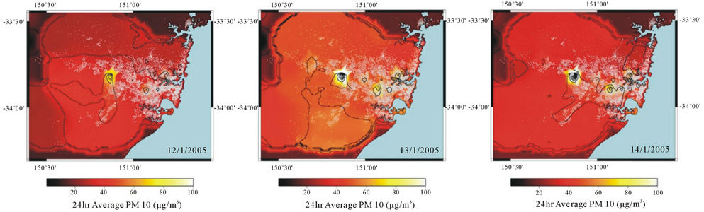
Figure 3. Average distribution of PM10 between 12/1/2005 and 14/1/2005.
training); 6) Employment (attending work); and 7) Other (unclassified and unspecified activities).
Gender and age, determines the amount of time doing each of the above activities (see Table 1 for a breakdown). Individual time usage characteristics determined the amount of time an individual spent in a particular geographical region, and, hence, the length of exposure to pollutants at that location. Three of these activities (Personal care, Domestic activities and other) occur in and around the home.
Two activities required individuals to travel to another location to perform some of their tasks (e.g., work). Within the model, “work” and “school” occurs at placesof-work and school locations, for which individuals travelled from their homes in their census districts to those locations. Similar to above, travel to both work and education institutions was matched against patterns observed in the census.
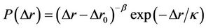
The remaining activities (Social and Community Interaction, and Recreation and Leisure), represent more general activates such as social gatherings, visiting friends, charity work, and visiting shopping centers. Given the many unknown factors that influence individual patterns of mobility (ranging from means of transportation, joband family-imposed restrictions, priorities and social preferences) we model these patterns as a truncated Lévy flight [9]:
 ,(1)
,(1)
where ,
,  km, and the cut-off value
 . This function specifically states that the probability of an individual travelling a distance
 , from their home, exponentially decays to a sharp cut-off of 80 km. Essentially, each person frequently makes short trips, and occasionally undertakes long distance travel, which we believe is a reasonable assumption for the Sydney metropolitan region.
2.2.3. Pollution-Dose Response Function
EpiCast-API provides a model of human movement through space and time, while TAPM provides information about the amount of pollution an individual is exposed to while undertaking various activities. To determine the effect of pollution on an individual, we need to: 1) assess the amount of pollution an individual was exposed to, and 2) analyze the health consequences arising from the exposure.
Here, we use the dose-response relations estimated by Ostro [10]. These response relations are derived from studies of US and UK cities. The health outcome for an individual i is:
 , (2)
, (2)
where  is the probability that person i will be affected by health outcome j,
  is the probability that on a given day, an individual will be affected by health outcome j given 1 μg/m3 of PM10, and
  is the level of exposure individual i has had to PM10. The value for Ei is:
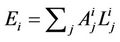 , (3)
, (3)
where  is the fraction of the total day spent by individual i performing activity j (see Table 1) and
  is the level of PM10, or other pollutant of interest, that individual i was exposed to at the location where activity j took place. Alternative versions of these equations are possible for other pollutants because some variables (e.g., maximum daily exposure) may be more important for determining health outcomes for those pollutants. For PM10, we assumed that the average exposure over the course of the day is the best indicator for determining health outcomes.
Following Ostro [10], we develop a series of health outcomes resulting from exposure to PM10. We analyze
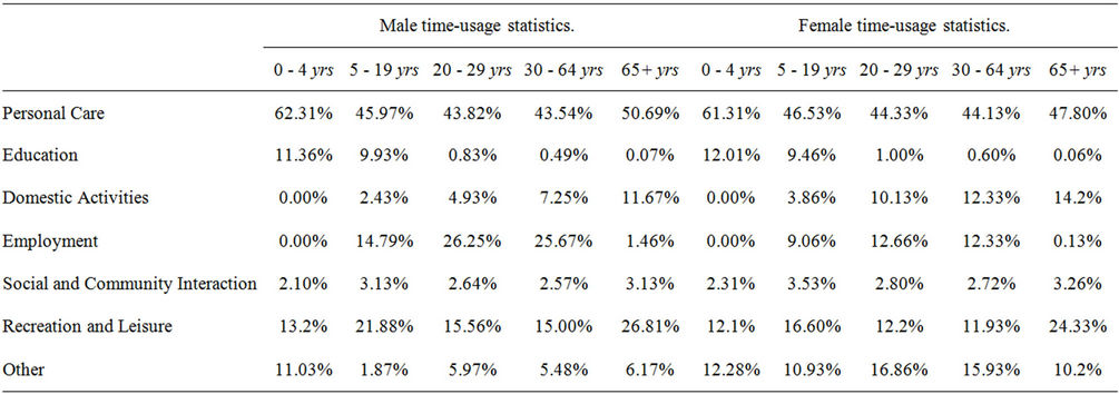
Table 1. Time usage statistics.
mortality, respiratory hospital admissions, and emergency room visits. High, central, and low estimates of the rate of occurrence (attack rate) for each health outcome, that represent the mean and 95% confidence intervals, provide us with a mechanism for estimating the uncertainty or error bounds on the estimate of affected people. The rates of each health outcome are as follows:
Mortality (M). The central estimate for the number of cases of mortality due to PM10 was expressed as
 , (4)
, (4)
where C is the crude coefficient (6.74 deaths per 1,000 people, per year, in Australia, 2010). The high, central, and low morbidity coefficient (mi) estimates are 0.13, 0.096 and 0.062 respectively. Thus the high, central and low morbidity coefficients per person per day per μg/m3 of PM10 are:
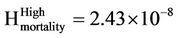 , (5a)
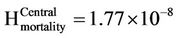 , (5b)
 . (5c)
It should be noted that, individuals who die are removed from the population for the remainder of the simulation.
Respiratory Hospital Admissions (RHA). RHA reflects severe afflictions that require the individual to be hospitalized. RHA includes hospitalizations for pneumonia, asthma, and bronchitis. The high, central, and low RHA coefficients per person, per day, per μg/m3 of PM10 are as follows:
 , (6a)
 , (6b)
 , (6c)
We assume that the estimated daily cost of a hospital admission is AUD $53,678 [11]. Length of hospital stay was randomly generated from a normal distribution with a mean of 10.13 days and a standard deviation of 2.2 days [10]. Hospitalized individuals are absent from work for the entire time they are in hospital. It is assumed that they return to work five days after their discharge.
Emergency Room Visits (ERV). ERV includes afflictions that require urgent attention, but do not require hospitalization (e.g., severe asthma attack). The high, central, and low ERV coefficients, per person, per day, per μg/m3 of PM10 were:
 , (7a)
 , (7b)
 , (7c)
The estimated cost of an emergency room visit was AUD $215 [12]. We assumed that individuals who visit the emergency room were absent from work for one day.
Once the probability of a particular health outcome was calculated, a value was randomly drawn from the distribution [0, 1]. If the randomly selected value was less than the probability of having a particular health outcome, then the agent was afflicted with that health outcome, and the outcome was recorded. In the case of mortality, the agent was removed from the simulation.
3. Scenarios, Simulations and Results
3.1. Scenarios
In assessing the impact of pollution control measures for Sydney, we developed a baseline scenario and three alternative pollution-change scenarios. The reference scenario represents the daily PM10 pollution level for Sydney for the year 2005. The remaining three alternatives are one pollution-reduction scenario and two pollutionincrease scenarios. In the reduction scenario PM10 is reduced by 50% while in the remaining scenarios PM10 levels are increased by 100% or 200%. We preserved the spatial structure of emission sources and dispersal in each scenario by using percentage changes in pollution levels.
3.2. Simulations and Results
For each of the scenarios outlined above, we constructed an ensemble of 100 realizations and averaged them for each scenario. Model output for each scenario included changes in mortality, respiratory hospital admissions, and emergency room visits (Tables 2-4 and Figures 4-6). In the remainder of this section, we will highlight the key results and findings; we will report low and high estimates for each health outcome, and for further detail the reader is directed to Tables 2-4. These high and low estimates relate to the high and low attack rates for each health outcome as detailed in §2.2.3. Where costs are reported all dollar values are listed in constant 2009 Australian dollars (AUD $).
3.2.1. Mortality
The first major impact we explore is the effect each scenario has on mortality. Mortality can be thought of as an important crude measure of the burden PM10 has on society. The baseline scenario recorded a low and high estimate for total deaths of 336 and 656 deaths (Table 2). The 50% reduction scenario produced a substantial reduction in the low and high estimates for the number of total deaths, 121 and 340 deaths. The two pollution increase scenarios produced substantially higher total death
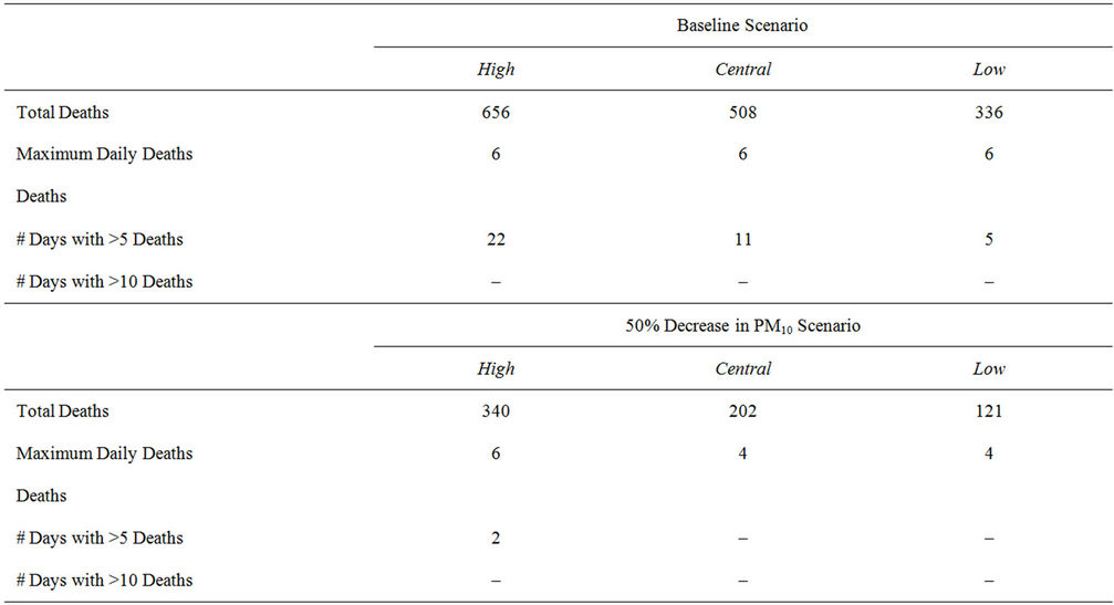
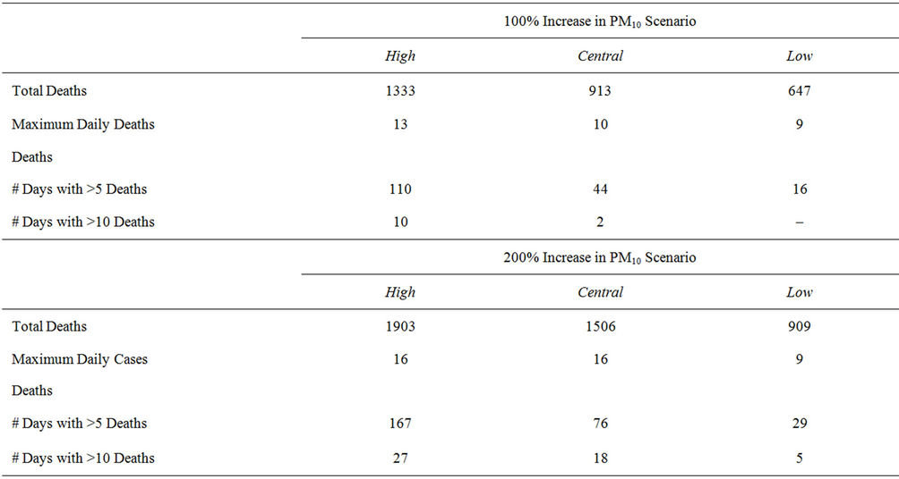
Table 2. Mortality for each air pollution scenario.
estimates than the baseline scenario. The 100% increase scenario generated low and high total death estimates of 647 and 1333 deaths. While the 200% increase scenario generated low and high total death estimates of 909, and 1903.
As these results illustrate, the scenarios exploring the effect of increased PM10 levels show a substantial negative impact on mortality. Also they illustrate the positive impact that continued efforts in maintaining or lowering air pollution levels can have on reducing the burden of mortality on society.
3.2.2. Respiratory Hospital Admissions
Respiratory hospital admissions can be thought of as a measure of burden placed on the health care system. Our results demonstrated significant daily effects on admissions to hospitals for respiratory disorders. The baseline scenario recorded low and high estimates of total admis-
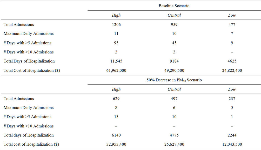
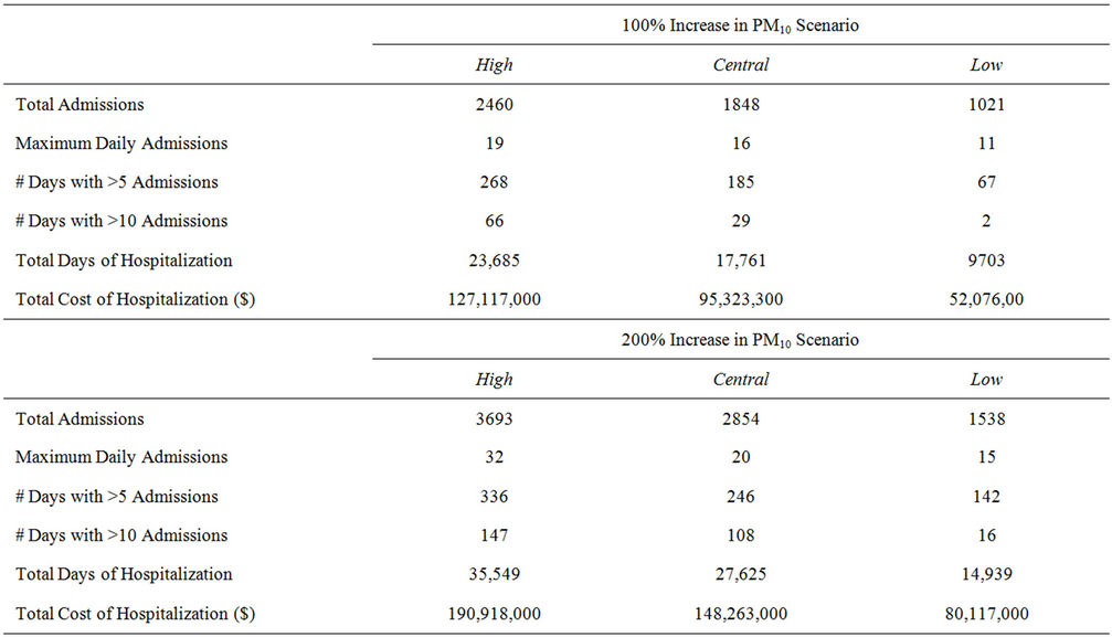
Table 3. Respiratory hospital admissions for each air pollution scenario.
sions of 477 and 1206 admissions (Table 3). The low and high estimates of the number of days with more than 5 admissions, was 9 and 93 days respectively. The low and high total days of hospitalization estimates are 4625 and 11,545 days and the associated costs of hospitalizetion are $24 million and $62 million respectively.
The 50% reduction in PM10, estimated the low and high total number of admissions to be 237 and 629. The low and high estimates of the number of days with 5 or more admissions are 5 and 8 days. The low and high total days of hospitalization estimates are 2244 and 6140 days and the associated costs of hospitalization are $12 million
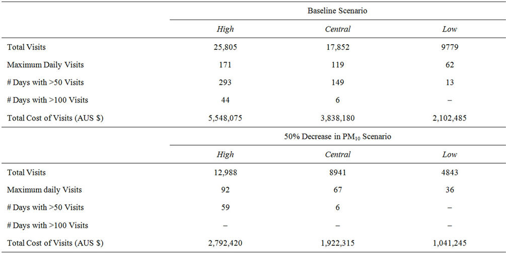
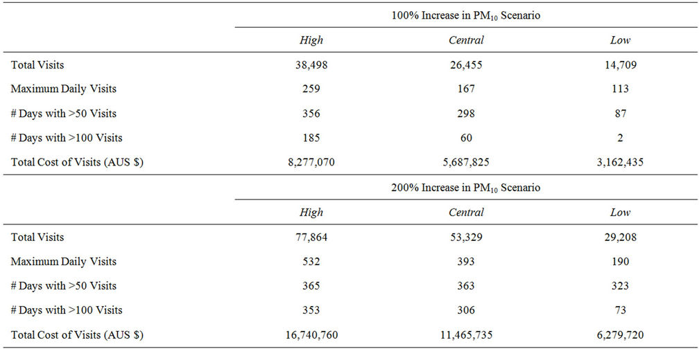
Table 4. Respiratory hospital admissions for each air pollution scenario.
and $33 million respectively.
The two pollution increase scenarios again show a substantial negative impact on respiratory hospital admissions. The 100% increase in PM10, estimated the low and high total number of admissions to be 1021 and 2460. The low and high estimates of the number of days with 5 or more admissions are 67 and 268 days. The low and high total days of hospitalization estimates are 9703 and 23,685 days and the associated costs of hospitalization are $52 million and $127 million respectively. Finally, the 200% increase in PM10, estimated the low and high total number of admissions to be 1538 and 3693. The low and high estimates of the number of days with 5 or more admissions are 142 and 336 days. The low and high total days of hospitalization estimates are 14,939 and 35,549 days and the associated costs of hospitalization are $80 million and $190 million respectively. The results illustrate that an increase in PM10 can substantially increase the pressure on hospitals, and incur a substantial cost to the health care sector.
3.2.3. Emergency Room Visits
The incidence of emergency room visits is an important indicator of immediate medical attention required due to
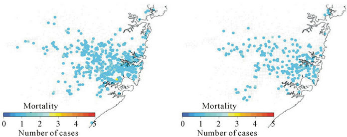
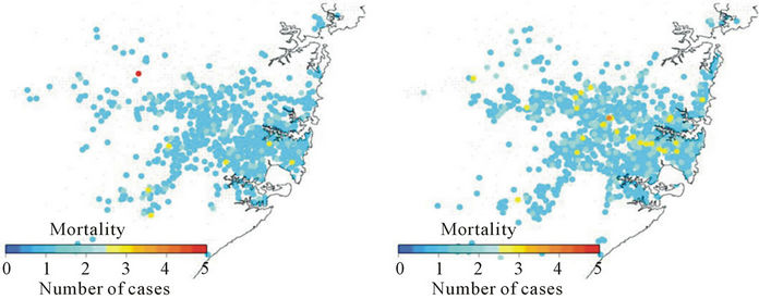
Figure 4. Spatial distribution of mortality cases resulting from contact with PM10 under each of the scenarios.
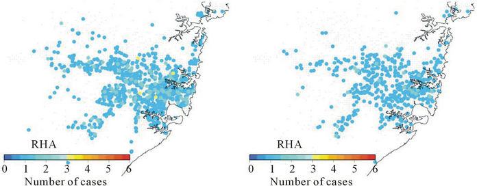
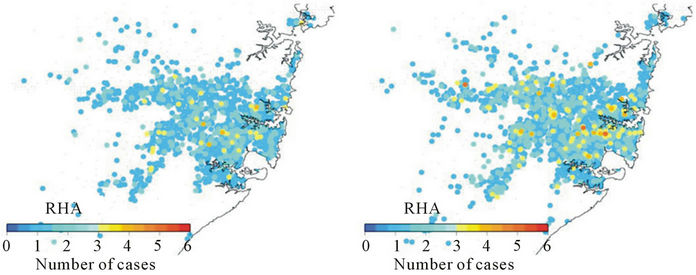
Figure 5. Spatial distribution of respiratory hospital admissions resulting from exposure to PM10 under each of the scenarios.
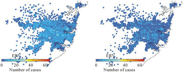
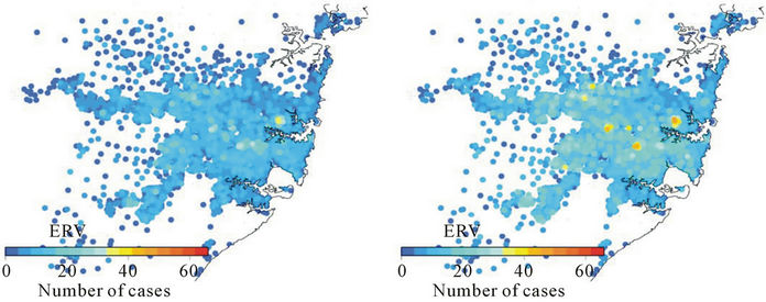
Figure 6. Spatial distribution of emergency room visits resulting from exposure to PM10 under each of the scenarios.
changes in PM10. For the baseline scenario, the high and low estimates of the total number of emergency room visits are 9779 and 25,805 visits (Table 4). Of particular interest when exploring the number of emergency room visits is the number of days with 50 or more visits. This is an indicator of the stress emergency medical facilities are placed under. The low and high estimates of the number of days with 50 or more emergency room visits for the baseline scenario are 13 and 293 days. Low estimates of the total cost of emergency room visits are $2.1 million, while high estimates place the cost at $5.5 million.
The low and high estimates of total emergency room visits for the 50% reduction scenario are 4843 and 12,988 visits. This is substantially lower than the results from the baseline scenario.
The low and high estimates for the number of days with 50 or more emergency room visits for the 50% reduction scenario are 0 and 59 days. This is a significant reduction in the burden on emergency medical facilities over the baseline scenario. Low estimates of the total cost of emergency room visits are $1 million, while high estimates place the cost at $2.7 million.
The pollution increase scenarios recorded low and high total emergency room visits of 14,703 and 38,498 visits; and 29,208 and 77,864 visits for the 100% and 200% increase scenarios respectively. The pollution increase scenarios also showed large increases in the burden on emergency rooms, with the low and high estimates for the number of days with 50 or more emergency room visits being 87 and 356 days respectively for the 100% increase scenario, and 323 and 365 days for the 200% increase scenario. Low estimates of the total cost of emergency room visits are $3.1 million and $6.2 million for the 100% and 200% increase scenarios respectively. While the high estimates for the total cost of emergency room visits for the two scenarios are $8.2 and $16.7 million for the 100% and 200% increase scenarios respectively.
3.2.4. Spatial Distribution of Impacts
The spatial distribution of mortality cases, hospital admission for respiratory disorder and emergency room visits associated with each scenario in the Sydney metropolitan region is presented in Figures 4-6. Analysis of the spatial patterns of the occurrence of each of the major health outcomes shows that the regions in Sydney that are most affected are those with lower socio-economic backgrounds. The many of the census districts most heavily affected have relatively “normal” levels of PM10. Further investigation shows that these census districts tend to be made up of single parent families, and those employed in sectors requiring semi or unskilled labor. The source of the exposure to PM10, is from a source outside their home environment.
3.2.5. Further Analysis
Finally, our simulation analysis clearly shows the adverse health impacts of potential increases in air pollution associated with PM10: higher mortality rates, and increased respiratory hospital admissions, emergency room visits, and health care costs. Furthermore, the number of days with lost productivity, for both those affected and their household caregivers, adds to the socio-economic impacts associated with potential increases in PM10 air pollution. These are important areas for further analysis in the future.
4. Concluding Remarks
The World Health Organization estimates that 2.4 million people will die each year from causes directly attributable to air pollution [13]. Short term health effects of air pollution include irritation to the eyes, nose, and throat; and upper respiratory infections such as bronchitis and pneumonia. Long term health effects include chronic respiratory disease, lung cancer, heart disease, and even damage to the brain, nerves, liver, and kidneys. Each of these health outcomes adds a direct cost to the health care sector and additional stress on the health care system (i.e., increased hospital admissions and emergency room visits), as well as indirect costs to the wider economy through factors such as lost labor from primary absenteeism (i.e., individuals who cannot work due to pollutionrelated illness), secondary absenteeism (i.e., individuals who cannot work because they are caring for someone who has a pollution-related illness), and restricted activity.
Despite developing national air quality standards for pollutants such as carbon monoxide, nitrogen dioxide, sulfur dioxide and lead, many countries including Australia still face major challenges from particulate pollution (for example, pollution caused by PM10 and PM2.5). Because emissions from commercial and other domestic sectors are growing in many regions, increasing their relative contribution to overall emissions, there is a continuing need to develop appropriate pollution mitigation and controls and standards.
The formation and evaluation of alternative environmental protection, emissions mitigation and control measure is a complex task. Often this is made even more difficult as:
• The number of possible control strategies is so large that it is not easy to evaluate all possible strategies to find the best strategy;
• The pollution control measures exist in a time varying environment and as a result an “optimal” solution we put in place today, to achieve a particular outcome, is far from optimal into the future;
• There may be many (possibly conflicting) objectives. For example, there may be a need to continue particular high polluting industries, while at the same time implement heavy clean air targets, and reduce medical expenditure; and
• The “final” policy is highly constrained. That is the final policy should satisfy many restrictions imposed by internal regulations, capacities, laws, technological constrains, preferences and social demands.
This highlights the increasing need for integrated tools that combine environmental, demographic and economic information to allow policy makers to evaluate alternative air pollution control scenarios. In this paper, we have outlined an agent-based modeling approach that can be used to help improve the capacity to evaluate alternative policy options for air pollution control. As discussed earlier, the analytical framework developed in this paper incorporates key relevant variables including population and demographic data, exposure-response relationships, and spatial variation in air quality.
We believe that the integrated analytical framework used in this paper can promote the development, analysis and synthesis of better information and knowledge about pollutants, exposure and impacts in order to improve public policy making. We have demonstrated this capability by analyzing the impacts of three illustrative scenarios involving the change in the levels of PM10 in the Sydney metropolitan region. The results of this scenario analysis highlight the fact that changes in PM10 pollutant levels could have considerable health implications and consequences.
Although the model implemented in this paper evaluates alternative air-quality scenarios for the Sydney metropolitan region, the model framework can be applied to any geographical area in the world. The main strengths of our integrated framework are: 1) treatment of individuals as a heterogeneous group; 2) explicit consideration of different characteristics of individuals including gender, age, family structure, occupation, location of residence and work, etc; 3) ability to explicitly accommodate individual behavior such as travel and interactions with others; and 4) the ability to assess responses to external stimuli (such as withdrawal from social and recreation activities due to high levels of pollution). It is important to recognize the data-intensive nature of the framework that requires data regarding human responses to pollutants. The availability of detailed air pollutant and population data has made it possible to study the impacts of air pollution in fine detail, although the lack of actual and detailed exposure-response relationships has been a constraint; and is an area that requires further attention and empirical work.
5. Acknowledgements
The authors acknowledge Tim Germann and John Finnigan for their assistance during this study. The authors would also like to thank Mark Hibbard, Martin Cope, and Sunhee Lee for providing the TAPM runs that this work was based on.
REFERENCES
- NSW Department of Environment, Climate Change and Water, “NSW State of the Environment 2009 Report,” Sydney, 2009.
- T. C. Germann, K. Kadau, I. M. Longini and C. A. Macken, “Mitigation Strategies for Pandemic Influenza in the United States,” Proceedings of the National Academy of Science, Vol. 103, No 15, 2006, pp. 5935-5940. doi:10.1073/pnas.0601266103
- D. Newth and D. Gunasekera, “Climate Change and the Effects of Dengue upon Australia: An Integrated Analysis of Health Impacts and Costs,” IOP Conference Series: Earth and Environmental Science, Vol. 11, 2010.
- M. Cope, S. Lee, J. Noonan, B. Lilley, D. Hess and M. Azzi, “Chemical Transport Model Technical Description,” Centre for Australian Weather and Climate Research, Melbourne, 2009.
- P. Hurley, “TAPM V4. Part 1: Technical Description,” CSIRO Marine and Atmospheric Research Paper No. 25, 2008. http://www.cmar.csiro.au/research/tapm/docs/tapm_v4_technical_paper_part1.pdf
- P. J. Hurley, W. L. Physick, and A. K. Luhar, “TAPM: A Practical Approach to Prognostic Meteorological and Air Pollution Modeling,” Environmental Modelling and Software, Vol. 20, No. 6, 2005, pp. 737-752. doi:10.1016/j.envsoft.2004.04.006
- Australian Bureau of Statistics, “2006 Census of Population and Housing,” 2006.
- Australian Bureau of Statistics, “How Australians Use Their Time, 2006,” 2008.
- M. C. González1, C. A. Hidalgo and A.-L. Barabási, “Understanding Individual Human Mobility Patterns,” Nature, Vol. 453, 2008, pp. 779-782. doi:10.1038/nature06958
- B. Ostro, “Estimating Health Effects of Air Pollution: A Methodology with an Application to Jakarta,” World Bank Policy Research Working Paper 1301, The World Bank, Washington DC, 1994.
- B. Jalaludin, G. Morgan, G. Salkeld, and C. Gaskin, “Health Benefits of Reducing Ambient Air Pollution Levels in the Greater Metropolitan Region,” NSW Department of Environment, Climate Change and Water and the NSW Department of Health, Sydney, 2010.
- Productivity Commission, Public and Private Hospitals, Research Report, Canberra, 2009.
- World Health Organization, “The Global Burden of Disease: 2004 Update,” World Health Organization, Geneva, 2008. http://www.who.int/healthinfo/global_burden_disease/GBD_report_2004update_full.pdf
NOTES
*Corresponding author.