Communications and Network
Vol. 4 No. 2 (2012) , Article ID: 19098 , 10 pages DOI:10.4236/cn.2012.42017
MAC-PHY Cross-Layer for High Channel Capacity of Multiple-Hop MIMO Relay System
Division of Physics Electrical and Computer Engineering, Graduate School of Engineering, Yokohama National University, Yokohama, Japan
Email: hiep@kohnolab.dnj.ynu.ac.jp
Received February 22, 2012; revised March 31, 2012; accepted April 24, 2012
Keywords: Multiple-Hop Relays System; Amplify-and-Forward; Optimization Distance; Optimization Transmit Power; MAC Layer Protocol; Infinite Antenna Number
ABSTRACT
For the high end-to-end channel capacity, the amplify-and-forward scheme multiple-hop MIMO relays system is considered. The distance between each transceiver is optimized to prevent some relays from being the bottleneck and guarantee the high end-to-end channel capacity. However, in some cases, the location of relays can’t be set at the desired location, the transmit power of each relay should be optimized. Additionally, in order to achieve the higher end-to-end channel capacity, the distance and the transmit power are optimized simultaneously. We propose the Markov Chain Monte Carlo method to optimize both the distance and the transmit power in complex propagation environments. Moreover, when the system has no control over transmission of each relay, the interference signal is presented and the performance of system is deteriorated. The general protocol of control transmission for each relay on the MAC layer is analyzed and compared to the Carrier Sense Multiple Access-Collision Avoidance protocol. According to the number of relays, the Mac layer protocol for the highest end-to-end channel capacity is changed. We also analyze the end-to-end channel capacity when the number of antennas and relays tends to infinity.
1. Introduction
Multiple-input multiple-output (MIMO) relay systems have been discussed in several literatures. Both the Gaussian MIMO relay channels with fixed channel conditions derive upper bounds and lower bounds that can be obtained numerically by convex programming. The upper bound and the lower bound on the ergodic capacity are found. In particular, for the case when all the nodes have the same number of antennas, the capacity can be achieved under the certain signal to noise ratio (SNR) condition [1-3]. Additionally, the ergodic capacity of the amplifyand-forward relay network is discussed. The links between the relay-transmitters and relay-receivers are assumed to be parallel [4] and serial [5,6]. Moreover, the endto-end channel capacity based on the different number of antennas at the transmitter, the relay and the receiver also has been evaluated [5,6]. However, the number of relays considered there (in [5] and [6]) is only one. The capacity of a particular large Gaussian relay network is determined by the limit as the number of relays tends to infinity. The upper bounds are derived from cut-set arguments, and the lower bounds follow an argument involving the uncoded transmission. It is shown that in case of interest, the upper and lower bounds coincide in the limit as the number of relays tends to infinity [7].
When the number of the relay antennas is less than the number of the transmit and receive antennas, the capacity of MIMO relay system is lower than that of the original MIMO system. Moreover, when the number of the relay antennas equals the number of the transmit and receive antennas or more, the MIMO relay system can provide the same average capacity as an original MIMO system. In other words, although the number of relay antennas is larger than the number of transmit and receive antennas, the capacity of MIMO relay system can’t exceed the capacity of original MIMO system [5,6,8-10].
Therefore, in order to achieve the high performance, the multiplehop relays system is considered. The diversity-multiplexing gain tradeoff (DMT) of multi-hop MIMO relay network with multiple antenna terminals in a quasi-static slow fading environment has also been considered. It is shown that the dynamic decode-andforward protocol achieves the optimal DMT if the relay is constrained to half-duplex operation. All the odd (or even) number hops is assumed to be operated simultaneously. However, the interference signal is assumed to be absent, and the perfomance based on a transmission protocol that only has two phases is analyzed [11]. The multiple-relay network, in which each relay decodes a selection of transmitted message by other transmitting terminals, and forwards parities of the decoded codewords, has been analyzed. This protocol improves the previously known achievable rate of the decodeand-forward strategy for multi-relay networks by allowing the relays to only decode a selection of messages from the relays with strong links to it [12].
However, in these papers the SNR at receiver(s) is assumed to be fixed and the location as well as the transmit power of each transmitter(s) are not dealt. In the multiple-hop MIMO relay system, when the distance between the source (Tx) and the destination (Rx) is fixed, the distance between the Tx to a relay (RS), RS to RS, RS to the Rx called the distances between transceivers, is shorten. Consequently, according to the number of relay and the location of the relays, the SNR and the capacity are changed. Hence, to achieve the high end-to-end channel capacity, the location of each relay meaning the distance between each transceiver needs to be optimized. We have analyzed the performance of half-duplex multiple hop relay system with the amplify-and-forward (AF) strategy [13]. We have obtained the high end-to-end channel capacity by optimizing the distance with equal transmit power. However, for achieving the higher endto-end channel capacity or in case the relay can’t be set at the desired location, the transmit power of each relay should be optimized. We propose the Markov Chain Monte Carlo method to optimize both the distance and the transmit power simultaneously. Additionally, the general transmission protocol on the Mac layer of multiplehop is analyzed based on the different propagation environment and the number of antennas at each relay. It is compared with Carrier Sense Multiple Access-Collision Avoidance protocol (CSMA-CA).
The rest of the paper is organized as follows. We introduce the concept of multiple-hop MIMO relays system in Section 2. Section 3 shows the optimization method for distance and the transmit power. The Mac layer protocol is described in Section 4. The end-to-end channel capacity of system with infinite number of antennas and relays is analyzed in Section 5. Finally, Section 6 concludes the paper.
2. Multiple-Hop MIMO Relays System
The multiple-hop MIMO relays system is described in details in [13]. However we choose some important parts to help the reader understand easier.
2.1. Channel Model
Figure 1 shows m relays intervened MIMO relay system. Let M, N and  denote the number of the antenna at the
 ,
,  and
and , respectively. The

Figure 1. Concept of multiple-hop relay system.
distance between each transceivers is denoted by . The distance between the
  and the
  is fixed as
 . The
. The  and all the relays employ amplify-and-forward strategy. Mathematical notations used in this paper are as follows. x and X are scalar variable, x and X are vector variable or matrix variable,
  is conjugate transpose.
In order to easily describe, the ,
,  are also be denoted as the
  and
and , respectively. Since the path loss is taken into consideration, channel matrix is a composite matrix and we model as
 , of which
  and
and  represent the path loss and the channel matrix between the
  and the
 , respectively. The path loss is described in details in the following section.
  is a matrix with independent and identical distribution (i.i.d.), zero mean, unit variance, circularly symmetric complex Gaussian entries.
We assume that the transmit power of the  (
( ) and the total transmit power of relays (
 ) are fixed and are not affected by the change in the number of relays and antennas at each relay. In order to simplify the composition of relay and demonstrate the effect of optimizing the distance and the transmit power of each relay, we assume that the transmit power of each relay is equally divided into each antenna and the number of antenna in each relay is the same. Moreover, the perfect channel state information is assumed to be available to both the transmitter and the receiver, and the zero forcing algorithms are applied. Consequently, the capacity of downlink (from
  to
to ) in multiple-hop relay systems is expressed as [13]
 (1)
(1)
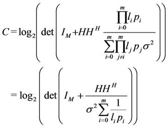
here, H denotes the channel matrix of the system and be represented as ;
;  represents the transmit power of one antenna of
 .
.
However, in this system all the relays transmit the signal in the same time, with full allocation time and the interference signal is assumed to be absent. Hereafter, this system is called the ideal system, and the end-to-end channel capacity is called the ideal end-to-end channel capacity.
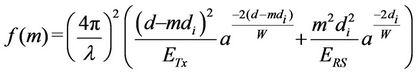
Let
 (2)
(2)
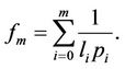
As the definition of  above,
  becomes a Gaussian matrix regardless of the number of relay, the distance between each transceiver and the transmit power of each relay. It means that the end-toend channel capacity is only abode by f(m). Therefore, function f can be considered instead of the end-to-end channel capacity. In order to achieve the high end-to-end channel capacity, the function f has to be minimized. In [13], the distance between each transceiver is optimized when the transmit power of each relay is assumed to be equal. In this paper we are going to optimize both the transmit power and the distance simultaneously.
2.2. Path Loss
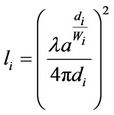
As in Equation (1), the system channel matrix is proportional to  and
and . Therefore, the path loss plays an important role in the channel model. Since there are a lot of obstacles in propagation environment, such as huge building and so on, it is necessary to consider the path loss as being attenuated by the reflection. The power of signal is reduced corresponding to the transmission distance and the number of reflections. An amount of the reduction by one time reflection is called reflection factor. Naturally, the reflection factor is changed according to the shape of obstacles, the angle of reflections and so on. However, in this paper, the reflection factor of all reflections is assumed to be the same and denoted by a. The path loss is expressed as [14]
 (3)
(3)
of which  is the reflected number while the signal is transmitted between
  and
and . Additionally, the propagation environment is specified by the propagation environment coefficient. The propagation environment coefficient W is defined as the average distance from a relay/Tx or from a reflection point to the next reflection point or the next relay/Rx. In other words, it is the average of line-of-sight (LOS) distance between each transceiver. Therefore, the reflected number between each transceiver can be expressed as
  and the path loss in Equation (3) can be rewritten as
 (4)
(4)
3. Optimizing Transmit Power and Distance
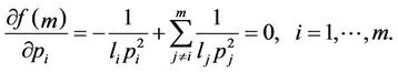
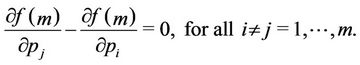
3.1. Optimizing Transmit Power of Each Relay
The partial differential equation of  with respect to
  is expressed as
 (5)
(5)
Thus,
 (6)
(6)
Therefore, the relation between any two transmit powers is described as
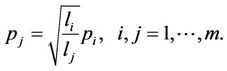 (7)
(7)
Moreover, the total transmit power of relays  is fixed and the transmit power of all antennas in the same relay is the same,

Thus, the optimized transmit power can be obtained,
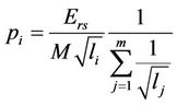 (8)
(8)
3.2. Optimizing Distance and Transmit Power
The function f(m) can be rewritten by
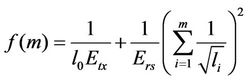 (9)
(9)
For analyzing performance of this system easily, let W denote the average of  (
( , meaning the average of LOS distance between the Tx and
 . Let
. Let  change from 1 to m, the partial differential equation of
  with respect to
  becomes,
 (10)
(10)
Since the type of the partial differential equation of  is the same for all
 , one of the solutions of this equation is
 . Substituting for Equation (8), we can obtain the optimized transmit power as
 (11)
(11)
Since the end-to-end channel capacity with average W is almost the same as end-to-end channel capacity with difference,  , W can be used instead of
  [13]. Additionally, one solution of
  can be specified as
 . Substituting
  in
in ,
,  becomes a function of
 .
.
 (12)
(12)
Let
 .
.
The Taylor expansion is applied for  and
and . Thus,
  becomes a polynomial equation and di can be obtained by solving
  by using the Galois theory [15].
To analyze the performance of this system with difference  is the same. The Taylor expansion is applied for the term
 . Then, the partial differential equation of
  with respect to each
  is obtained, and each
  can be obtained by solving
 . However, in this case, we have used the Taylor expansion, solving the partial differential
  times to obtain each
 .
.
3.3. The System with Interference
When the system has no control on the Mac layer or has incompletely controlled, the interference signal is presented. The received signal at the  is considered. The RSi simultaneously receives the desired signal
  from the
  and the interference signal
  from the
 . Actually, the
  receives the interference signal not only from the
  but also from all the previous relays. However, the interference signals from the other relays are weaker than the interference signal from the
 . Hence the interference signals from the other relays can be ignored and the received signal at
  is expressed as
 (13)
(13)
Consequently, the end-to-end channel capacity can be expressed as
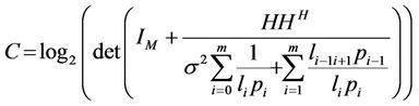 (14)
(14)
In comparison with the end-to-end channel capacity without interference, the term of interference
 is added. The transmit power and the distance can be optimized as the case of the system without interference. However, the optimization distance of system with difference
 , especially the system with interference, is complicated. In order to easily optimize the distance and the transmit power simultaneously, the Markov chain Monte Carlo (MCMC) algorithm is proposed.
3.4. Markov Chain Monte Carlo
The MCMC algorithm is used to find the optimum state of the distance and the transmit power, that has the minimum of f. The MCMC algorithm is shown in Figure 2 and explained as follows.
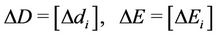
Let D, E denote  distance vector and transmit power vector, respectively.
 (15)
(15)
Step 1: The initial value of function f is given by equaling all the distances between each transceiver and all the transmit powers of each relay. Let the initial value of f be min.
Step 2:  and
and  are defined as the distance and the transmit power to next state.
  and
and  are
are  vector as,
here,  and
and  are the random values subject to
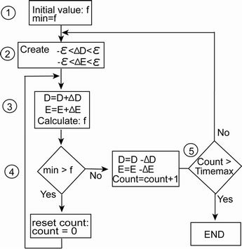
Figure 2. MCMC algorithm.
 (16)
(16)
Step 3: Calculate the function f after shifting the distance vector and the transmit power vector to the next state.
Step 4: compare value of f at new state and min, if minf, count is reset and go back to step 3. Otherwise, let the distance and the transmit power come back to the previous state and count increases by 1.
Step 5: If count > timemax, the current state is the optimum state, the current distance and the transmit power are optimum and the algorithm is finished. Otherwise, go back to step 2.
Since the distance and the transmit power are optimized by shifting randomly, the MCMC method requests a high timemax and small  for convergence. It means that the MCMC method requests enough a number of samples to find the optimized state of the distance and the transmit power. At step 4 of the MCMC algorithm, the count of sample is reset every time, the better state of the distance and the transmit power is found. Thus, actually, the number of samples is much higher than timemax. Additionally, by shifting the distance and the power randomly, MCMC method can avoid the local optimum and obtain the global optimum. In comparison with the mathematical method, MCMC algorithm is easier to control both of the distance and the transmit power, especially when
  is different and the interference signal is presented. However, the MCMC algorithm requests to run in computer and appropriate
  and
and . The terms
  and
and  are depended on the system model, such as the propagation environment coefficient of each node, the number of relay node, and so on. We compare the ideal end-to-end channel capacity of mathematical method and MCMC method in Figure 3. According to Figure 3, for this system model with W = 500 m or over, the calculation result is the same when
  is smaller than
 , and
, and  is larger than 10,000. Therefore,
  and
and  are applied.
3.5. Numerical Evaluation
The system parameter summarized in Table 1 is an example for evaluation.
Since the end-to-end channel capacity in the different propagation environment is evaluated in [13], in this paper, only different  propagation environment with average being 500 m is expressed. The optimized distance and the optimized transmit power in case of interference presence are shown in Figure 4. The short distance corresponding to the transmit power is provided
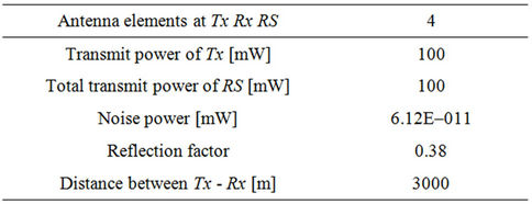
Table 1. Numerical parameters.
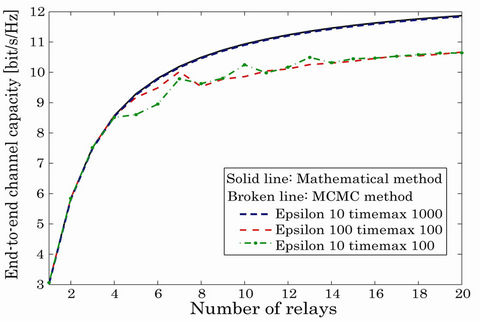
Figure 3. Comparing end-to-end channel capacity of mathematical method and MCMC method with some epsilons and timemaxs.
for the short  environment. It means that the optimization distance can prevent some relay from being a bottleneck of the system and the performance of each relay is guaranteed.
The channel capacities of the average distance, the transmit power and the optimized distances, the transmit power are compared in Figure 5. The channel capacities of the average distance, the transmit power are deteriorated rapidly by bottleneck. On the other hand, since the amplify-and-forward scheme is applied for all relays, the performance of relays forwarding to  is deteriorated. However, according to optimizing the distance and the transmit power; the performance of relays is decreased slowly. As a result, the end-to-end channel capacity of the optimized distance and the transmit power is higher than that of the average distance and transmit power.
Figure 6 shows the end-to-end channel capacity with and without optimizing the distance and the transmit power based on the number of different relays. The optimal transmit power is quite effective. However, optimizing both of the distance and the transmit power demonstrates that the end-to-end channel capacity can be much higher. Moreover, there are a number of the optimum relays for the largest end-to-end channel capacity. It can be explained that when the number of the relays is small, the distance between each transceiver is large, thus the end-to-end channel capacity is low. The end-to-end channel capacity is increased when the
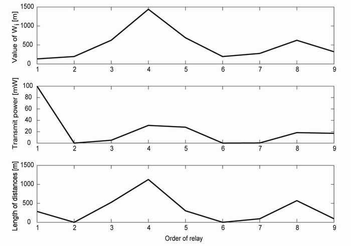
Figure 4. Optimized distance and transmit power in system with different Wi and presence of interference signal, the relay number is 8.
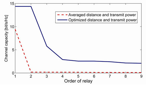
Figure 5. Comparing the end-to-end channel capacity of optimized and averaged distance and transmit power in different Wi system with interference signal, the relay number is 8.
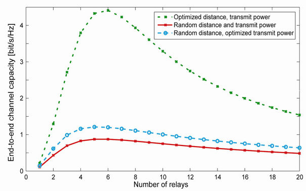
Figure 6. end-to-end channel capacity of system with and without optimized distance and transmit power.
number of the relays increases. However, when the number of the relays is large, the distance is shortened; hence the power of desired signal is higher. However, the power of interference signal also goes higher. As a result, the signal to interference noise ratio (SINR) is small. Therefore the end-to-end channel capacity is decreased.
Since the interference signal is presented in the system without control, the SINR is decreased, meaning the endto-end channel capacity is decreased, especially when the number of the relays is large. In order to maintain the higher performance, the transmission must be controlled on the Mac layer.
4. Mac Layer Protocols
4.1. Multiple-Phases Transmission
The transmission of each relay in the system can be divided into the multiple-phases. The relays in the same phases transmit the signal in the same time and the allocation time ( ). In the other phases, the relay keeps the silence or receives the signal. Since the neighbor relay transmits the signal in different phases, the interference signal is weaker than that of the system without control.
The Figure 7 shows 2 phases and 3 phases transmission protocol. The 2 phases transmission protocol is explained as follows. The even-number relays and the odd-number relays transmit the signal in phase 1 and phase 2, respectively. The allocation time for each phase is equal.
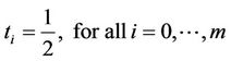 (17)
(17)
The end-to-end channel capacity in case the transmission of all relays is controlled on MAC layer, is denoted by . Thus, the end-to-end channel capacity is expressed by
 (18)
(18)
here C is the end-to-end channel capacity with the interference mentioned in Section 3.3. However, the interference signal comes from the third previous relay. Hence, the term of interference is changed as
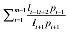 .
.
Similarly, the allocation time, the end-to-end channel capacity and the term of interference of n phases protocol are expressed by
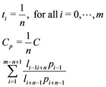 (19)
(19)

Figure 7. 2 phases and 3 phases transmission protocol.
The optimized distance and transmit power can be obtained the same as the method mentioned above.
4.2. Carrier Sense Multiple Access-Collision Avoidance
There are some protocols of time division multiple accesses (TDMA), such as carrier sense multiple access with collision detection (CSMA-CD), carrier sense multiple access-collision avoidance (CSMA-CA) and so on. Because of commonplaceness of CSMA-CA, the proposed general Mac layer protocol is compared to CSMA-CA.
For collision avoidance, in CSMA-CA protocol, each relay transmits the signal in the different allocation time. Moreover, the waiting time is set at each relay for detecting the transmission in system. Therefore, in unit time, the allocation time that each relay transmits the signal, is less than . Therefore, the maximum of end-to-end channel capacity becomes as,
 (20)
(20)
here C denotes the end-to-end channel capacity without interference mentioned in Section 2.
On the other hand, due to applying AF scheme, the SNR and the channel capacity of  decrease as much as
  being higher. Hence, the last relays become the bottleneck of system. In order to achieve the higher endto-end channel capacity, the allocation time for each relay should be optimized. (In this paper, we only consider the allocation time, the appropriate modulation and the code word are left to future work.) The maximum of endto-end channel capacity is obtained when
here  is the channel capacity without interference of
 . Therefore,
 (21)
(21)
and the optimized allocation time is expressed as
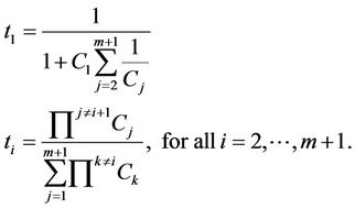 (22)
(22)
In this case, the maximum of end-to-end channel capacity is obtained by
 (23)
(23)
In Equation (22), the denominator of the optimized allocation times is the same, thus the allocation time only depends on the numerator. Moreover, the numerator is the product of channel capacity of all relays except for its own channel capacity. It means that the higher channel capacity of the relay achieves, the smaller allocation time is divided. Therefore, by appropriating the modulation and code word, the transmission rate of all relays is equal and the higher end-to-end channel capacity can be achieved. The result is shown in the next section.
4.3. Numerical Evaluation for Control Transmission
End-to-end channel capacity with and without control on the Mac layer is shown in Figure 8. For all cases, such as 2 phases, 3 phases, 4 phases, without control, CSMA-CA, we find the optimum number of relays which achieves the highest end-to-end channel capacity. The reason is explained in the previous section. However, the optimum number of relays for each case is different. When the number of relays is small, the distance between each transceiver is large. Therefore, the power of interference signal is low and hence the end-to-end channel capacity without control is high. Moreover, when the number of relays is large, the power of interference signal increases. Therefore, the system with Mac layer protocol in multiple phases demonstrates the effect. For achieving the high end-to-end channel capacity, the Mac layer protocol should be changed corresponding to the number of relays.
The end-to-end channel capacity of CSMA-CA with the optimized allocation time is higher than that of CSMA-CA with the average allocation time. However, although the interference signal is absent, the average allocation time for each relay is much smaller than the allocation time of the proposed general Mac layer protocol, the end-to-end channel capacity is much lower.
5. End-to-End Channel Capacity for Infinite Antennas Number and Relays Number
5.1. Infinite Antennas Number
Although the number of antenna at each relay is assumed to be equal, the transmit power of each antenna is depended on the number of antennas. When the number of antenna decreases, the transmit power of each antenna increases, hence the power of received signal included the interference signal is increased. However, the term of interference described in the previous section is not depended on the number of antenna. Additionally, the difference of end-to-end channel capacity among all protocols is the term of interference. On the assumption that all antennas at one relay are equal, the end-to-end chan-
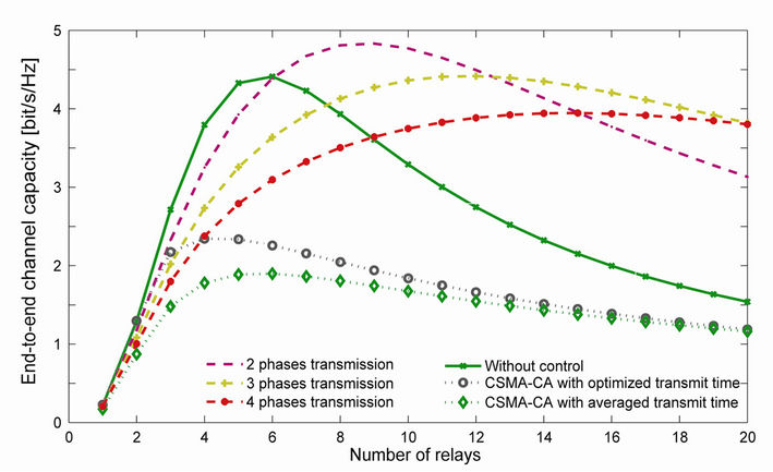
Figure 8. End-to-end channel capacity of system with and without control.
nel capacity of n phases transmission system can be rewritten based on the transmit power of each relay as
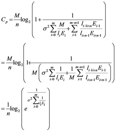 (24)
(24)
here e denotes the Napier’s constant.
5.2. Infinite Relays Number
However, the end-to-end channel capacity of all protocols decreases when the number of relays increases (Figure 8). If the number of relays also tends to infinity, the distance between each transceiver becomes small enough to assume that  is one regardless of
 . Thereforethe distance and the transmit power can be easily optimized because of disusing Taylor expansion.
 (25)
(25)
Substituting to Equation (24), the limitation of end-toend channel capacity is changed as
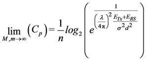 .
.
When a number of the antennas and the relays tend to infinity, the end-to-end channel capacity of all protocols converges to a certain value regardless of the propagation environment. However, the end-to-end channel capacity depends on the number of the transmission phases, it is decreased when transmission phase increases.
6. Conclusions
In this paper, we analyzed the end-to-end channel capacity of multiple-hop MIMO relays system with amplifyand-forward scheme. For the high end-to-end channel capacity, the cross-layer between the Physical layer and the Mac layer is considered. On the Physical layer, both the transmit power and the distance are optimized simultaneously by the mathematical method and MCMC algorithm. On the Mac layer, the general transmission protocol for multiple-hop relay system is proposed. We also optimize the allocation time for each relay in CSMA-CA strategy. The optimized allocation time CSMA-CA indicates the effect on end-to-end channel capacity. However, in order to achieve the high end-to-end channel capacity, the appropriate protocol is dependent on the number of relays, the propagation environment and so on. The endto-end channel capacity when the number of antennas at each relay and the number of relays tends to infinity, is examined.
However, in this paper, we only proposed the Mac layer protocol, the appropriate modulation and code word are not considered. In the future, the concrete system will be described and the appropriate modulation and code word will be examined. Additionally, the dependence on frequency of path loss and the full-duplex multiple-hop relay system also will be analyzed.
REFERENCES
- B. Wang, J. Zhang and A. host-Madsen, “On the Capacity of MIMO Relay Channel,” IEEE Transactions on Information Theory, Vol. 51, No. 1, 2005, pp. 29-43. doi:10.1109/TIT.2004.839487
- D. S. Shiu, G. J. Foschini, M. J. Gans and J. M. Kahn, “Fading Correlation and Its Effect on the Capacity of Multi-Element Antenna Systems,” IEEE Transactions on Communications, Vol. 48, No. 3, 2000, pp. 502-513. doi:10.1109/26.837052
- D. Gesbert, H. Bolcskei, D. A. Gore and A. J. Paulraj, “MIMO Wireless Channel: Capacity and Performance Prediction,” Global Telecommunications Conference, San Francisco, 27 November-1 December 2000, pp. 1083- 1088.
- Y. b. Liang and V. Veeravalli, “Gaussian Orthogonal Relay Channels: Optimal Resource Allocation and Capacity,” IEEE Transactions on Information Theory, Vol. 51, No. 9, 2005, pp. 3284-3289. doi:10.1109/TIT.2005.853305
- K.-J. Lee, J.-S. Kim, G. Caire and I. Lee, “Asymptotic Ergodic Capacity Analysis for MIMO Amplify-and- Forward Relay Networks,” IEEE Transactions on Communications, vol. 9, No. 9, 2010, pp. 2712-2717.
- S. Jin, M. R. McKay, C. j. Zhong and K.-K. Wong, “Ergodic Capacity Analysis of Amplify-and-Forward MIMO Dual-Hop Systems,” IEEE Transactions on Information Theory, vol. 56, No. 5, 2010, pp. 2204-2224. doi:10.1109/TIT.2010.2043765
- M. Gastpar and M. Vetterli, “On the Capacity of Large Gaussian Relay Networks,” IEEE Transactions on Information Theory, vol. 51, no. 3, 2005, pp. 765-779. doi:10.1109/TIT.2004.842566
- M. Tsuruta and Y. Karasawa, “Multi-Keyhole Model for MIMO Repeater System Evaluation,” Electronics and Communications in Japan, vol. 90, no. 10, 2007, pp. 40-48.
- D. Chizhik, G. J. Foschini, M. J. Gans and R. A. Valenzuela, “Keyholes, Correlations, and Capacities of Multi-Element Transmit and Receive Antennas,” IEEE Transactions on Wireless Communications, Vol. 1, No. 2, 2002, pp. 361-368. doi:10.1109/7693.994830
- G. Levin and S. Loyka, “On the Outage Capacity Distribution of Correlated Keyhole MIMO Channels”, IEEE Transactions on Information Theory, Vol. 54, No. 7, 2010, pp. 3232-3245. doi:10.1109/TIT.2008.924721
- D. Giindiiz, M. A. Khojastepour, A. Goldsmith and H. V. Poor, “Multi-Hop MIMO Relay Networks: DiversityMultiplexing Trade off Analysis,” IEEE Transactions on Wireless Communications, Vol. 9, No. 5, 2010, pp. 1738- 1747.
- P. Razaghi and W. Yu, “Parity Forwarding for Multiple-Relay Networks,” IEEE Transactions on Information Theory, Vol. 55, No. 1, 2009, pp. 158-173. doi:10.1109/TIT.2008.2008131
- P. T. Hiep and R. Kohno, “Optimizing Position of Repeaters in Distributed MIMO Repeater System for Large Capacity,” IEEE Transactions on Communications, Vol. 93, No. 12, 2010, pp. 3616-3623.
- N. Kita, W. Yamada, A. Sato, “Path Loss Prediction Model for the Over-Rooftop Propagation Environment of Microwave Band in Suburban Areas (in Japanese),” IEEE Transactions on Communications, Vol. 89, No. 2, 2006, pp. 115-125.
- H. M. Edwards, “Graduate Texts in Mathematics: Galois Theory,” Springer, New York, 1997.