Atmospheric and Climate Sciences
Vol.4 No.4(2014), Article
ID:49833,15
pages
DOI:10.4236/acs.2014.44049
Study of Weak Intensity Cyclones over Bay of Bengal Using WRF Model
Radhika D. Kanase, P. S. Salvekar
Indian Institute of Tropical Meteorology, Pune, India
Email: radhikakanase@gmail.com
Copyright © 2014 by authors and Scientific Research Publishing Inc.
This work is licensed under the Creative Commons Attribution International License (CC BY).
http://creativecommons.org/licenses/by/4.0/


Received 25 June 2014; revised 30 July 2014; accepted 29 August 2014
ABSTRACT
Numerical simulations of four weak cyclonic storms [two cases of pre-monsoon cyclones: Laila (2010), Aila (2009) and two cases of post-monsoon cyclones: Jal (2010), SCS (2003)] are carried out using WRF-ARW mesoscale model. Betts-Miller-Janjic (BMJ) as cumulus parameterization (CP) scheme, Yonsei University(YSU) planetary boundary layer (PBL) scheme and WRF single moment 6 class (WSM6) microphysics (MP) scheme is kept same for all the cyclone cases. Three two-way interactive nested domains [60 km, 20 km and 6.6 km] are used with initial and boundary conditions from NCEP Final Analysis data. The model integration is performed to evaluate the track, landfall time and position as well as intensity in terms of Central Sea Level Pressure (CSLP) and Maximum Surface Wind speed (MSW) of the storm. The track and landfall (time and position) of almost all cyclones are well predicted by the model (except for SCS cyclone case) which may be because of the accurate presentation of the steering flow by CP scheme. Irrespective of season, the intensity is overestimated in all the cases of cyclone, mainly because of the lower tropospheric and mid-tropospheric parameters are overestimated. YSU PBL scheme used here is responsible for the deep convection in and above PBL. Concentration of frozen hydrometeors at the mid-tropospheric levels and thus the latent heat released during auto conversion of hydrometeors is also responsible for overestimation of intensity.
Keywords:WRF-ARW Model, BMJ-YSU-WSM6 Combination, Pre and Post Monsoon Severe Cyclonic Storms

1. Introduction
Tropical Cyclones (TCs) are among the most devastating weather systems on the Earth. They cause considerable damage and destruction to lives and property due to strong gale winds, torrential rain and associated storm surge. India has a coastal line of 7600 km. Every year India experiences pre and post monsoon cyclones. Though general movement of the TCs is well known, it is desirable to have timely and reasonably accurate prediction of the tracks and intensities of such cyclones for effective implementation of the disaster mitigation. To improve the prediction, there is need of basic understanding of physics and dynamics involved in the genesis, intensity change, structure and track of tropical cyclone. The concept of Conditional Instability of Second Kind (Charney and Eliassen [1] ) indicated that cyclonic inflow in lower tropospheric boundary layer is essential for development of TCs. Gray [2] indicated that developing and non-developing cyclones are associated with different upper tropospheric circulation patterns e.g. non-developing TCs have uni-directional upper tropospheric flow which causes vertical shear above the cloud clusters relatively strong and the developing TCs normally have multidirectional out flow that results in weak vertical shear above the cyclones. The study of Holland and Merrill [3] concluded that not only upper tropospheric interactions but also the inner core convective heating may directly affect intensity change while lower tropospheric interactions will produce a size change which may indirectly affect the intensity or strength of Tropical cyclone. Craig and Gray [4] showed that the intensification of numerically simulated tropical cyclones is due to Wind Induced Surface Heat Exchange (WISHE). Holland [5] demonstrated that nonlinear combination of two processes: 1) an interaction between the cyclone and its basic current (steering current) and 2) an interaction with the Earth’s vorticity field, is responsible for movement of TCs.
With the advancement in the computer technology, several simulation studies have been conducted to study the TCs over the NIO using high resolution mesoscale models (Pattanayak and Mohanty [6] ; Deshpande et al. [7] [8] ; Trivedi et al. [9] ; Osuri et al. [10] [11] ; Bhaskar Rao et al. [12] ; Srinivas et al. [13] [14] ; Raju et al. [15] , Mukhopadhyay et al. [16] ). These studies are based on evaluating the model performance with respect to physics sensitivity, resolution, initial conditions and impact of data assimilation on the track and intensity forecast of very severe cyclones. In all the above studies, scientists have attempted simulation of strong tropical cyclones with rapid intensification. However, there is another class of TC which does not reach the stage of very severe cyclonic storm but attains lesser intensity, named as weak cyclones [Sever Cyclonic Storms (SCS) and Cyclonic Storms (CS)]. These weak cyclones, due to their slow motion and quasi-stationary nature, cause very heavy rainfall and in turn large amount of damage to the property. Very few studies have focused on simulating the weak intensity storms (Osuri et al. [11] , Srinivas et al. [17] ), but the detailed evolutions of structural changes in the genesis parameters during development of the storm are hardly addressed.
In the literature it is found that YSU as Planetary Boundary Layer (PBL) scheme and WSM6 as Microphysics scheme (Li and Pu [18] , Efstathiou et al. [19] , Tao et al. [20] , Mukhopadhyay et al. [16] ) and BMJ as Cumulus scheme (Kanase and Salvekar [21] ) give better track and intensity simulation of tropical cyclones. Therefore, here instead of testing the different combinations of physical parameterization, the combination (BMJ-YSUWSM6) is kept fixed for numerical simulation of four severe cyclonic storms Aila, Laila, Jal and SCS (Dec- 2003 cyclone has no specific name hence designated as SCS) during pre-and post monsoon season over Bay of Bengal (BoB). The changes in the vertical structure of the severe cyclonic storms, according to region as well as season, at the mature stage are also studied with the help of time evolution of different dynamic and thermodynamic genesis parameters. We also tried to find out the possible reason for the failure of this combination for the track of SCS cyclone.
2. Data and Methodology
2.1. Model Description
The non-hydrostatic fully compressible Advanced Research Weather Research and Forecasting (WRF-ARW) model version 3.2.1 developed by National Center for Atmospheric Research(NCAR) is suitable for a broad range of applications, such as idealized simulations, parameterization research, data-assimilation research and real-time numerical weather prediction (Skamarock et al. [22] ). The parameterization scheme for cumulus, microphysics and planetary boundary layer (PBL) used in the present study are given below.
Betts-Miller-Janjic (BMJ) cumulus scheme is based on the Betts-Miller convective adjustment scheme (Betts [23] ; Betts and Miller [24] ) with modifications introduced by Janjic [25] . This scheme removes the conditional instability in each grid column and adjusts the vertical profile of temperature and specific humidity towards a reference profile. This scheme triggers convection when a parcel (which is lifted moist adiabatically from the lower troposphere to a level above the cloud base) becomes warmer than the environment. WRF Single Moment 6 class (WSM6) microphysics scheme has six classes of hydrometeors i.e. Ice, snow, graupel, cloud water, rainwater and water vapor. Modifications from Hong et al. [26] , Houze et al. [27] , Tripoli and Cotton [28] have eventually resulted in reducing the cloud ice and increasing the snow at colder temperatures. Yonsei University (YSU) PBL scheme includes an explicit representation of entrainment at the PBL top which is derived from large eddy modeling (Hong and Pan [29] ). It has the capability to remove the influence of convective velocity on the surface stress, which will alleviate a daytime low-wind speed bias. Details are available in Hong and Lim [30] .
2.2. Data Used
The National Center for Environmental Prediction Final Analysis (NCEP-FNL) 1˚ × 1˚ data with Real Time Global (RTG) sea surface temperature is used as the initial and boundary conditions which are updated at every 6hr interval. The initial conditions are such chosen that for each case the model integration is started at least 24 hrs prior to the formation of Depression. For pre-monsoon cyclone Laila and Aila, model integration is started from 00UTC 16 May 2010 and 00UTC 24 May 2009 respectively and for post-monsoon cyclone Jal and SCS, it is started from 00UTC 03 Nov. 2010 and 00UTC 10 Dec. 2003 respectively. Jal cyclone is advected from northwest Pacific, so the system is already in the depression stage when it reached over the Indian region. Hence for Jal cyclone alone, the initial condition is chosen in such a way that the model is integrated at least 24hrs before intensifying into deep depression. The model integration is carried out 12 hrs beyond the observed landfall for all the cases. The model is run with three interactive domains of 60, 20 and 6.6 km and 31 vertical levels. Horizontal domain varies for each cyclone case (The details are available in Table 1).
3. Brief Description of Severe Cyclonic Storms
3.1. Laila
The cyclone “Laila” which formed during May 2010 is the first pre-monsoon severe cyclone that crossed Andhra Pradesh coast after 1990. Under the influence of onset of southwest monsoon over Andaman Sea and adjoining south BoB, the low level circulation turned to be a low pressure area on 12UTC 16 May with center near 9.0˚N/90.5˚E. It concentrated into depression on 06UTC 17 May and further into deep depression on 12UTC 17 May over southeast BoB, about 850 km east-southeast of Chennai. It moved westward and intensified into cyclonic storm at 00UTC 18 May, near 11.5˚N/86.5˚E with Central Sea Level Pressure (CSLP) of 998 hPa and Maximum Surface Wind speed (MSW) of 18 m·s−1. The cyclone further intensified into severe storm on 06UTC19 May and attained its maximum intensity of CSLP 986hPa and MSW 29 m·s−1 upto 09UTC 20 May. Cyclone moved slowly during landfall at Andhra Pradesh coast near Bapatla between 1100 and 1200UTC 20 May 2010. It caused heavy rainfall over coastal Andhra Pradesh and Tamil Nadu and flooding and damage along its path. The significant feature of the system is that it lay very close to the coast after landfall maintaining cyclone intensity for about 12 hrs after landfall (RSMC [31] ).

Table 1. Intensity, landfall Time and landfall position error of four cyclones.
3.2. Aila
According to RSMC [32] , under the influence of increased low level convergence due to the onset of SW monsoon over Andaman Sea and adjoining south BoB on 20 May 2009, a low pressure area is developed over the southeast BoB on 22 May morning. Under favorable conditions, like warmer sea surface temperature (SST) and low vertical wind shear, it concentrated into depression and further into deep depression at 03UTC 24 May near 18˚N/88.5˚E. Continuing its northerly movement, on 12UTC 24 May, it reached to the cyclonic storm stage. With CSLP of 974 hPa and MSW 29 m∙s−1, it attained its severe cyclonic storm stage at 0600 UTC 25 May over northwest BoB near 21.5˚N/88.0˚E close to Sagar Island and after couple of hours the system crossed West Bengal coast close to the east of Sagar Island. Immediately after landfall it has its maximum intensity with CSLP of 967 hPa and MSW as 31 m∙s−1 at 0900UTC. Under the influence of cyclone Aila, widespread rain/ thundershowers with scattered heavy to very heavy rainfall and isolated extremely heavy rainfall (≥25 cm) occurred over Orissa on 25 May and over West Bengal and Sikkim on 25 and 26 May. The special features of the cyclone Aila is, its northerly movement throughout its life period and its rapid intensification just prior to landfall. It maintained its cyclonic intensity up to 15 hours after landfall.
3.3. Jal
A severe cyclone “Jal” over the BoB is the remnant of a depression which moved from the northwest Pacific Ocean to the Bay of Bengal across Thailand. It concentrated into deep depression on 00UTC 5 Nov. 2010 near 9.0˚N/88.5˚E and further intensified into severe cyclone on 2100UTC 5 Nov and lay centered around 10.0˚N/ 86˚E, with maximum intensity of CSLP 988 hPa and MSW 31m∙s−1 for 12hrs from 12UTC 6 Nov. It weakened into a cyclonic storm at 0600 UTC 7 Nov. over southwest BoB about 250 km east-southeast of Chennai and further into a deep depression on 12UTC 7 Nov. near 13.0˚N/81˚E. It crossed north Tamilnadu-south Andhra Pradesh coast, close to the north of Chennai near 13.3˚N/80.3˚E around 1600 UTC 7 Nov. It continued to move west-northwestwards, further weakened into a depression at 0300 UTC and into a well marked low pressure area over Rayalseema and adjoining south interior Karnataka at 0600 UTC 8 Nov. Rainfall occurred at most places with heavy to very heavy fall at a few places over north Tamil Nadu, Puducherry, coastal Andhra Pradesh, Rayalseema, south Interior Karnataka and coastal Karnataka. The salient feature of the cyclone Jal is that it weakened into deep depression over the sea before the landfall (RSMC [31] ).
3.4. SCS
A low pressure area formed over the southeast Bay of Bengal and adjoining Indian Ocean on 8 Dec 2003 persisted for two days over the same area and then developed into well-marked low pressure area by 11 Dec morning. It concentrated into a depression near 4.5˚N/90.5˚E at 1200UTC 11 Dec. The system moved in a northwesterly direction and reached to the cyclonic storm at 1200UTC 13 Dec. With Maximum intensity of CSLP- 992 hPa, MSW-28 m·s−1, it remains in severe cyclone stage from 1200UTC 14 Dec. to 1800UTC 15 Dec. It made landfall near Machilipatnam around mid-night on 15 Dec. After landfall the system weakened into a cyclonic storm and further into Depression on 16 evening. Under the influence of this system heavy to very heavy rainfall occurred over Andaman and Nicobar Islands during the initial stages and over north Andhra Pradesh during the time of landfall. The special feature of SCS is the longer duration of severe cyclonic stage for about 30hrs (RSMC [33] ).
4. Results and Discussion
The outer domain of 60 km chosen for each case is given in the Table1
4.1. Initial Condition in Terms of Horizontal Surface Wind Fields
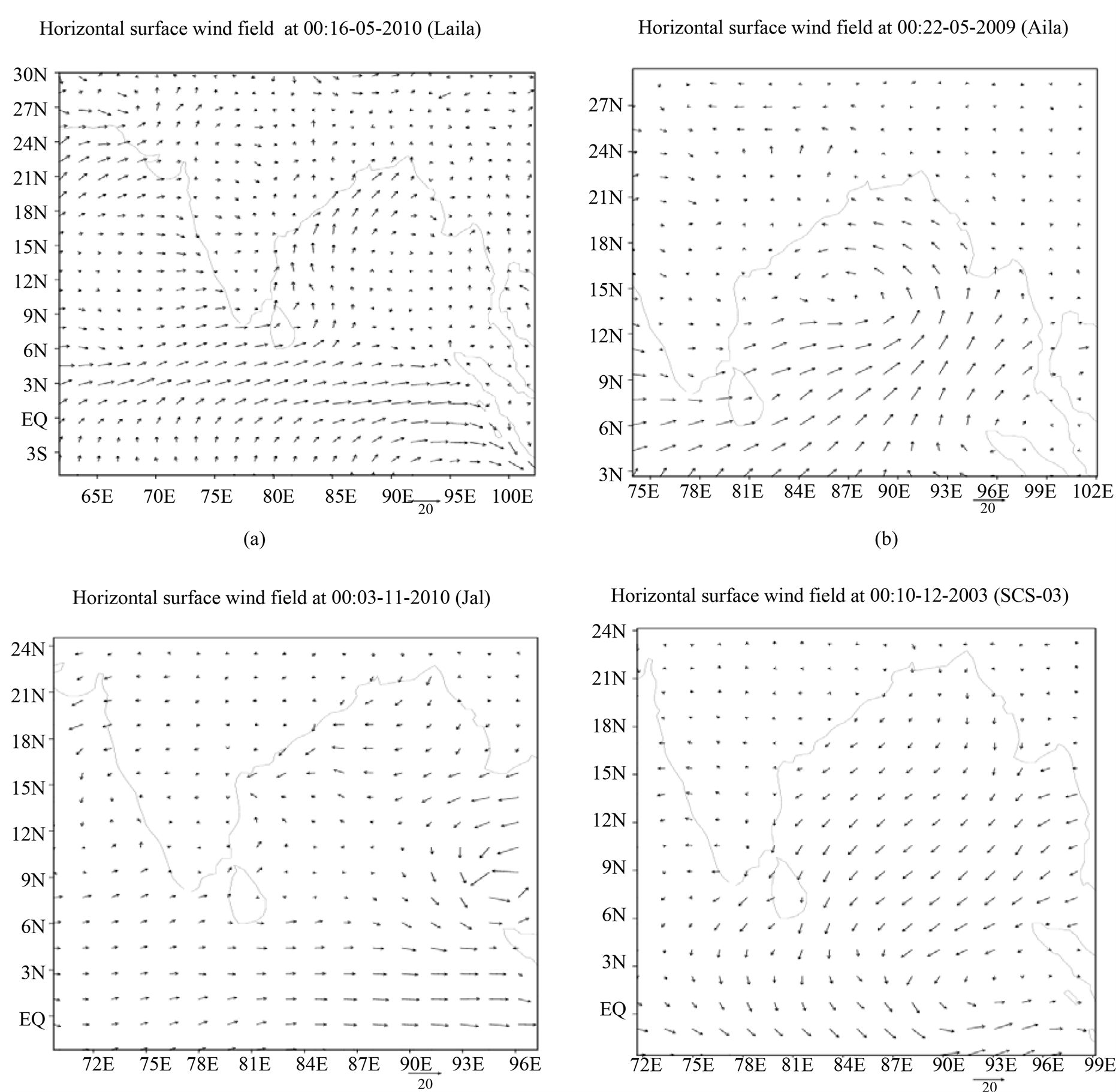
Figure 1 shows the initial horizontal wind fields for the four cyclones. For cyclone Laila, the initial condition (00UTC 16 May 2010) is 12 hrs prior to the formation of low and thus as shown in Figure 1(a), slight circulation in the region 6˚E - 15˚N and 80˚E - 95˚E is observed. In the case of cyclone Aila, the low pressure area (00UTC 22 May) is already formed and this initial condition is relatively closer to the Depression stage, so the well organized vortex with strong winds to the right side of the vortex (Figure 1(b)) is clearly depicted over 12˚N - 18˚N
 (c) (d)
Figure 1. Initial Horizontal wind fields as initial conditions form NCEP-FNL data set for cyclone: a) Laila at 00UTC 16th May 2010; b) Aila at 00UTC 22nd May 2009; c) Jal at 00UTC 3rd Nov 2010; d) SCS at 00UTC 10th Dec 2003.
and 84˚E - 90˚E. For Jal cyclone, the initial wind field at 00UTC 3Nov corresponds to the depression stage. Therefore, the stronger winds with the well organized vortex are clearly seen in Figure 1(c). For SCS, the model integration is started from 00UTC 10 Dec 2003. The low pressure is already formed on 8 Dec and it took about 3 days to intensify into the depression. Therefore, the slight circulation over the region 0˚N - 6˚N and 90˚E - 99˚E for cyclone SCS is clearly seen (Figure 1(d)). Thus starting from the initial feeble circulation, the model is integrated and its surface as well as upper air features are studied in detail.
4.2. Track and Intensity
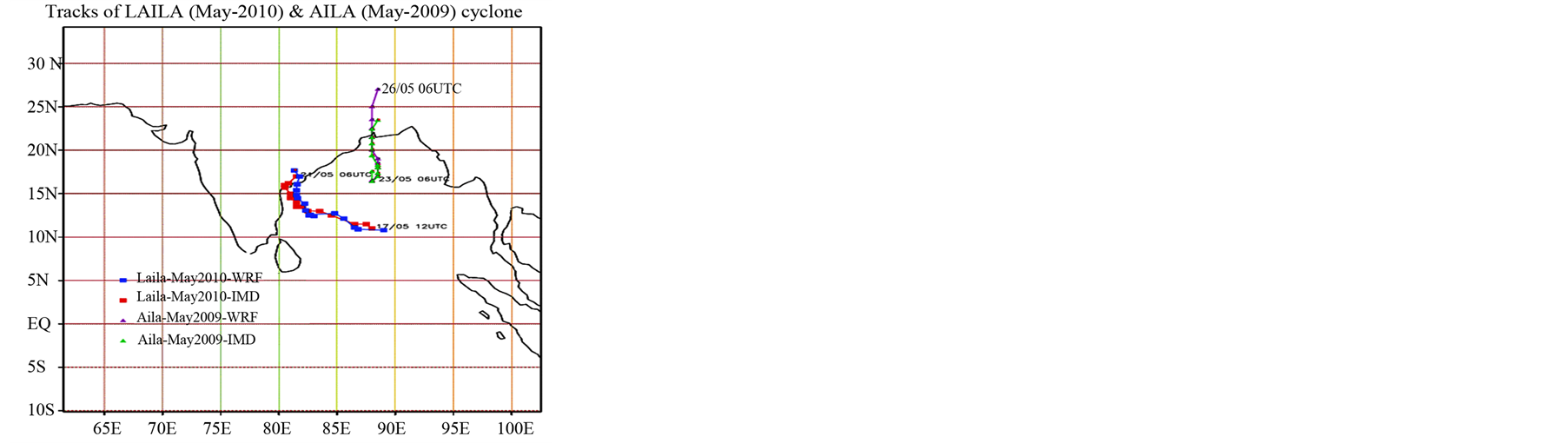
Figure 2(a) shows the simulated surface track of pre-monsoon cyclones along with IMD observed track. The track of both the cyclones Laila and Aila seems to be overlapped on IMD observed track. To understand the time evolution of track error, variation of track error is plotted in Figure 2(d). For cyclone Laila the track error is within the range 50 - 150 km and for cyclone Aila, initial 200 km track error decreases continuously up to 54
 (a)
(a)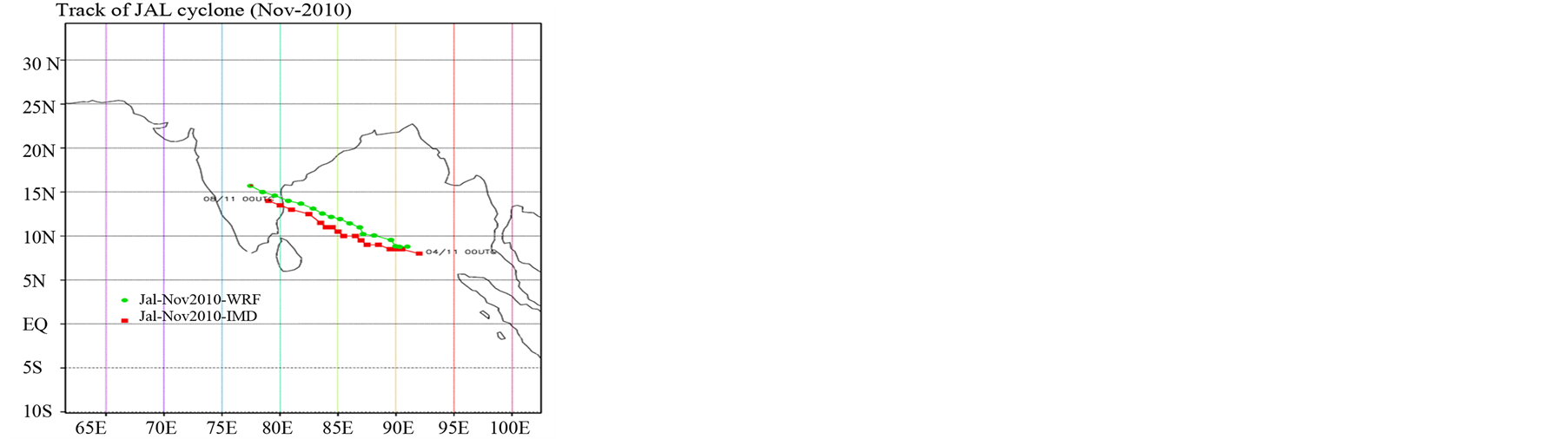 (b)
(b)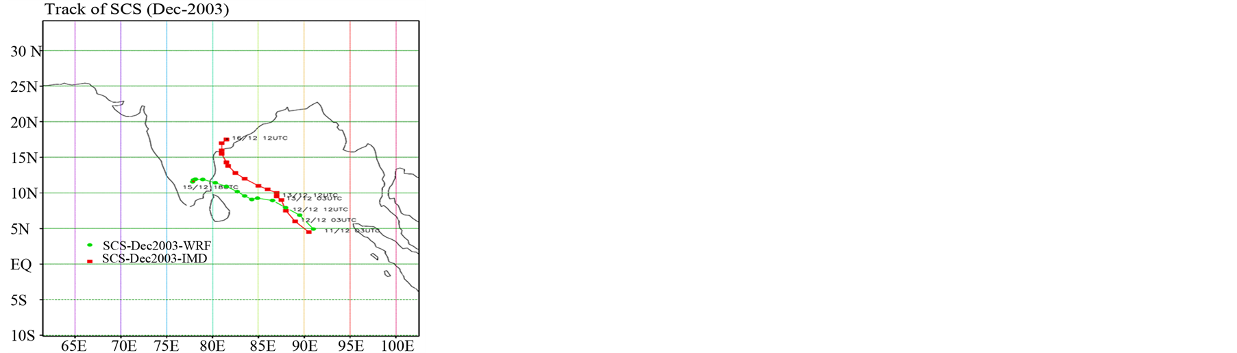 (c)
(c)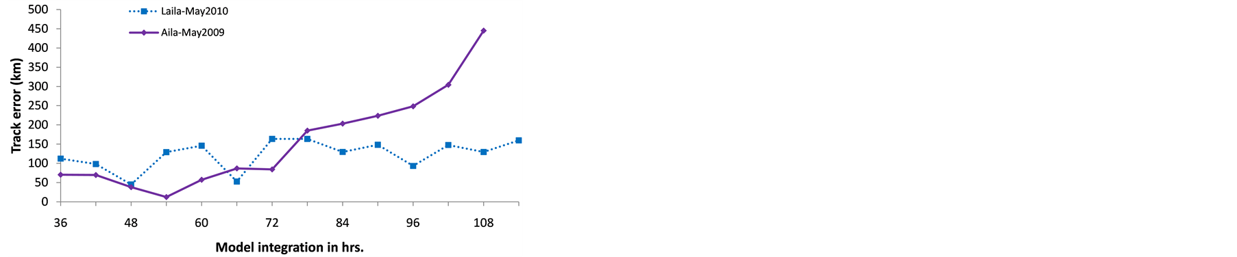 (d)
(d)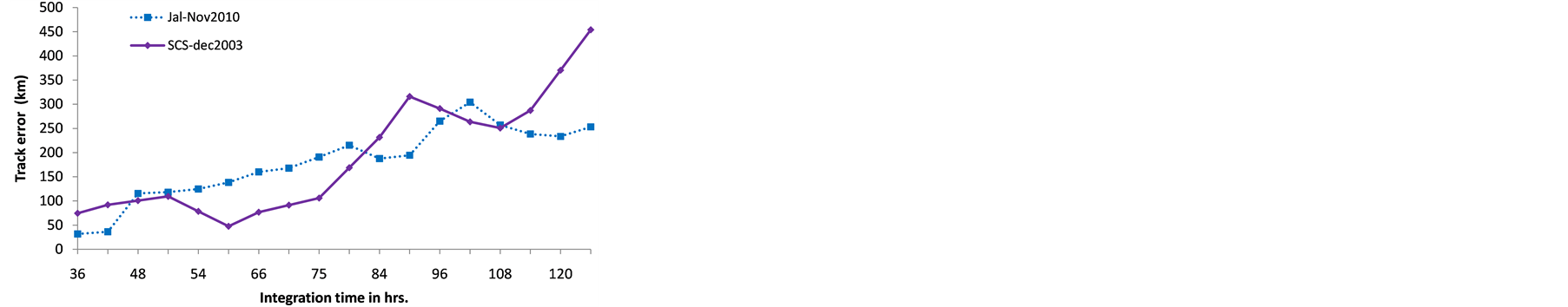 (e)
(e)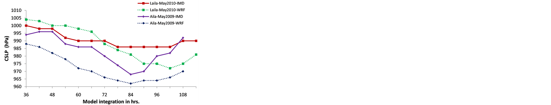 (f)
(f)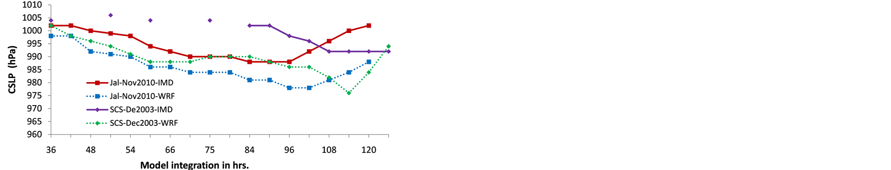 (g)
(g)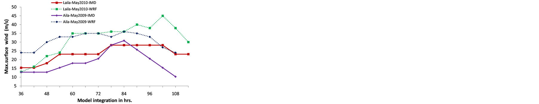 (h)
(h)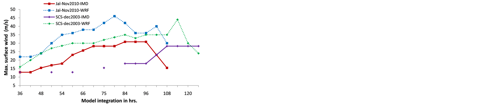 (i)
(i)
Figure 2. Track of a) Laila and Aila, b) JAL and c) SCS. Track error in km for d) Pre-monsoon, e) Post monsoon cyclones. Variation of CSLP in hPa for f) Pre-monsoon, g) Post monsoon cyclones. Variation of MSW in m/s for h) Pre-monsoon, i) Post monsoon cyclones.
hrs of integration period with minimum value of 24 km, but thereafter it continuously increases till dissipation of the system and attains it maximum value of 450 km. The initial decrease and then increase in the track error for Aila may be due to the slow translational speed of model cyclone as compared with the translational speed of observed cyclone (figure not shown). The track of post-monsoon cyclone JAL and SCS is shown in Figure 2(b) and Figure 2(c). In the case of Jal cyclone, the track is seen to be well simulated. Upto the landfall time (96 hrs of integration), the track error lies within the range 20 - 200 km and thereafter it increases up to 300 km (Figure 2(e)). For SCS cyclone, up to 75hrs of model integration, track error is less than 100 km, but thereafter it continuously increases with the maximum value of 600 km.
The proper upper level steering flow (mean wind between 300 and 100 hPa) is the main cause behind the better track prediction for all the cyclones (figure not shown). This upper level flow is north westerly for Laila cyclone, northward in the case of Aila cyclone and north westerly for Jal cyclone. This large scale environmental flow caused these three cyclones to move in the observed directions while this upper level steering current is initially for 2days in the north westerly direction and then in the westerly direction for SCS cyclone (figure not shown). Modeled SCS cyclone has moved towards the south-west than the observed cyclone. BMJ is a convective adjustment scheme, it adjusts the model pseudo adiabat with the reference lapse rate and during the adjustment process, it precipitate out the moisture. Weak intensity cyclones being quasi-stationary in nature, BMJ scheme may be able to produce proper steering flow as well as the large scale convection for these systems.
Intensity in terms of Central Sea Level Pressure (CSLP) and Maximum Surface Wind speed (MSW) for all the cyclones (Table 1) are discussed till India Meteorological Department (IMD) observations are available. The observed intensity (CSLP and MSW) with model simulated intensity values for Laila and Aila cyclone are shown in Figure 2(f) and Figure 2(h). The observed CSLP for Laila and Aila cyclone is 986 hPa and 968 hPa and the model simulated CSLP values are 972 hPa and 962 hPa respectively. For both the cyclones the intensity is overestimated but for the cyclone Aila it is relatively closer to the observed intensity. For cyclone Laila, intensity is underestimated up to 72 hrs and thereafter it is overestimated. But in the case of cyclone Aila, it is overestimated throughout the integration period. The intensity for the post monsoon cyclone is shown in Figure 2(g) and Figure 2(i). For both the cyclones, the intensity is overestimated throughout the period of model integration with the simulated values of CSLP are 978 hPa and 976 hPa respectively.
The model simulated Laila cyclone made landfall between 18UTC and 21UTC 20 May which is about 9 hrs late than the actual IMD observed landfall (12UTC 20 May) with landfall error of 140 km. For Aila cyclone, the simulated cyclone has landfall time in between 9-12UTC 25 May which is ~2 - 3 hrs late than actual IMD landfall with landfall error of 184 km. The observed landfall for Jal cyclone is around 16UTC 7 Nov 2010 and the model simulated landfall is between 09-12UTC which is 4 - 6 hrs early than the actual observed landfall. For SCS, the simulated landfall is between 18-21UTC 14 Dec 2003 which is 24 hrs delayed than the observed landfall. The error in the landfall position of Jal cyclone is 110 km and for SCS cyclone is 555 km. The landfall position error and landfall time for all the four cyclones are summarized in Table1
4.3. Illustration of Structure Change during Development and Possible Reasons behind Intensity Overestimation
The vertical structure of cyclones in terms of variation of horizontal wind speed and warm core (i.e. temperature anomaly) is discussed at the corresponding mature stage of cyclones. For pre-monsoon cyclones Laila and Aila, the mature stage is at 06UTC 20 May 2010 and 09UTC 25 May 2009. For post monsoon cyclones, Jal and SCS, the mature stage is at 06UTC 7 Nov 2010 and 18UTC 14 Dec 2003. With the help of temporal evolution of different possible dynamical and thermodynamical parameters such as lower level relative vorticity ζ, relative humidity and temperature (Kotal et al. [34] ) we tried to find out the reason behind the success/failure of BMJ-YSU-WSM6 combination in overestimating the intensity of the cyclones. The factors affecting the cyclone intensity are divided into lower tropospheric parameters and Mid-tropospheric parameters. We will discuss these parameters in following sections.
4.3.1. Lower Tropospheric Parameters Affecting the Cyclone Intensity
The horizontal wind structure at the mature stage for all the cyclones can be clearly seen in the Figure 3. For cyclone Laila, the calm winds with the magnitude < 5 m∙s−1 are clearly seen at the center of cyclone surrounded by very strong winds on both the sides of center of cyclone. The maximum winds are found to be throughout the boundary layer and are not restricted to the 850 hPa level. For cyclone Aila, at 09UTC 25 May (Figure 3(b)),
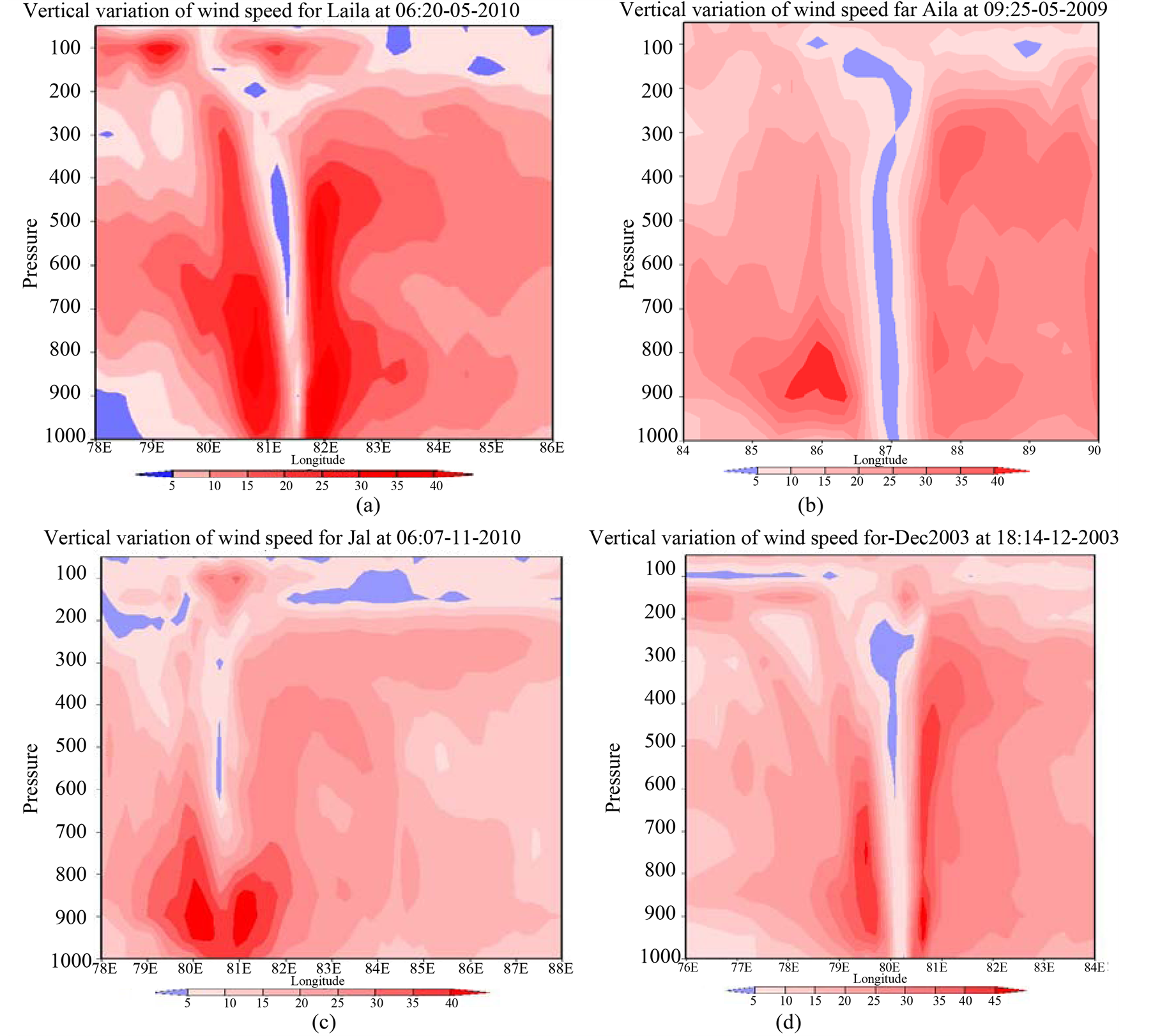
Figure 3. Vertical variation of horizontal wind speed (m/s) for a) Laila at 06:20-05-2010; b) Aila at 09:25-05-2010; c) Jal at 06:07-11-2010; d) SCS at 18:14-12-2010.
the calm winds are clearly seen at the center with surrounding strong winds having maxima at 850hPa level. These strong winds are observed to the west side of the cyclone center. Here the extension of eye region in the horizontal direction is seen to be less than half degree and the vertical extent of the calm region is from surface upto the upper troposphere. For the post monsoon cyclone Jal (Figure 3(c)) strong winds are restricted to the lower troposphere while eye is observed in the mid-tropospheric level. For SCS cyclone, the wind structure at mature stage shows that the eye is extended to the 200 hPa level (Figure 3(d)). The eyewall has one maximum at 950 hPa on one side and another maximum at 750 hPa on other side of cyclone center. Therefore the time evolution of the low level relative vorticity (ζ850) is obtained throughout the cyclone development and dissipation stage (Figure 4(a)). For each individual cyclone, the range of relative vorticity at 850 hPa level differs from each other depending upon the intensity simulated by the model. Intercomparison between the relative vorticity with the intensity variation then it is found that upto 00UTC of 19 May, the intensity is underestimated by the model and thereafter it is overestimated which closely matches with the relative vorticity behavior. The decrease in the relative vorticity after the mature stage corresponds to the decreased intensity.
For Aila cyclone, relative vorticity increases continuously from 20 × 10−5 to 160 × 10−5 s−1 upto 06UTC 24 May and then slowly decreases upto the landfall time and finally the vorticity value lies around 70 × 10−5 s−1 (Figure 4(b)). According to the observations (IMD report), the cyclone Aila is intensified just before the landfall. The model has captured this intensification just before the model landfall (Model landfall is ~2 to 3 hrs.
 (a)
(a)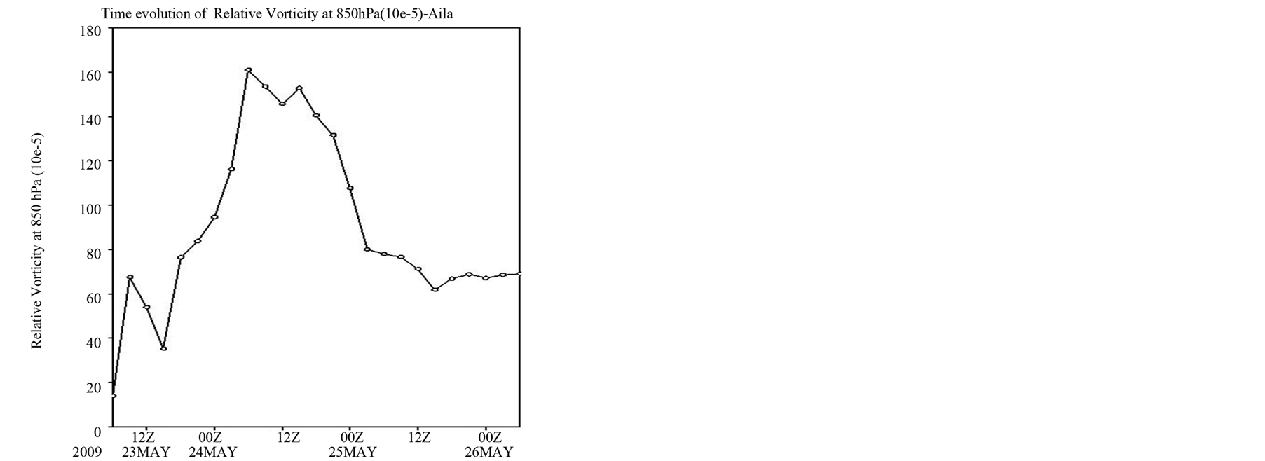 (b)
(b)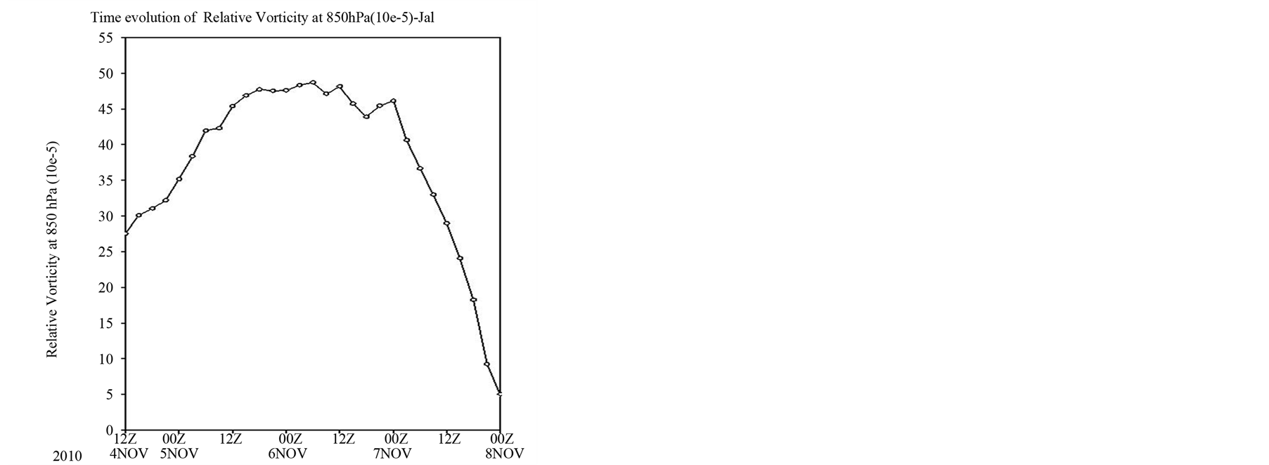 (c)
(c)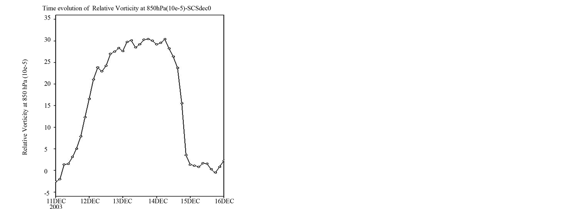 (d)
(d)
Figure 4. Time evolution of low level Relative Vorticity (10−5∙s−1) averaged over corresponding cyclone path for a) Laila (80˚E - 88˚E, 11˚N - 17˚N); b) Aila (88˚E - 89˚E, 16˚N - 28˚N); c) Jal (78˚E - 92˚E, 8˚N - 15˚N); d) SCS (80˚E - 90˚E, 4.5˚N - 17.5˚N).
delayed) and the observed as well as model mature stage is well matched. Also the comparable vorticity values after the landfall shows that the cyclone is not weakened immediately into LoPar and it sustained its cyclonic intensity upto 24 hrs of model landfall. For cyclone Jal, initially at 12UTC 4Nov, the low level relative vorticity is strong and it continuously increases upto 00UTC 7 Nov (Figure 4(c)) and rapidly decreases thereafter. The circulation vanishes completely at 00UTC 8 Nov as the time corresponds to the post landfall time. The upper level diverging fields are clearly depicted above 200 hPa level. Initially the anticyclonic circulation (Figure 4(d)) is observed at 00UTC of 11 Dec 2003, thereafter the cyclonic circulation increases and lies within the range 25 × 10−5 to 30 × 10−5 s−1 upto 00UTC of 14 Dec and then decreases rapidly as it approaches towards the land for cyclone SCS. The cyclone made landfall between 18-21UTC of 14 Dec and it immediately weakens (depicted from the zero vorticity values after landfall). The model simulated mature stage of this cyclone is at 18UTC of 14 Dec 2003. Intercomparison of the low level vorticity values among the four cyclones shows maximum for Aila and minimum for SCS cyclones.
YSU PBL scheme assumes deep mixing extended to the layer above the PBL top and thus moisture is transported upward through too deep of a layer. The strong vorticity variation and thus the strong winds in the boundary layer helped it to build deep convection during the development stage of the cyclones and is further supported by time evolution of mid-tropospheric relative humidity i.e. the difference between the relative humidity at 700 hPa - 500 hPa level (Figure 5). For all the cyclones, at the mature stage, the relative humidity at 700 hPa level is seen to be lowest with the corresponding increase in the relative humidity values at 500 hPa during developing stage and vice versa near the dissipating stage. This may be one of the reasons in overestimating the intensity for all cyclones.
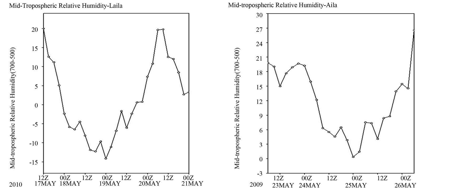 (a)
(a)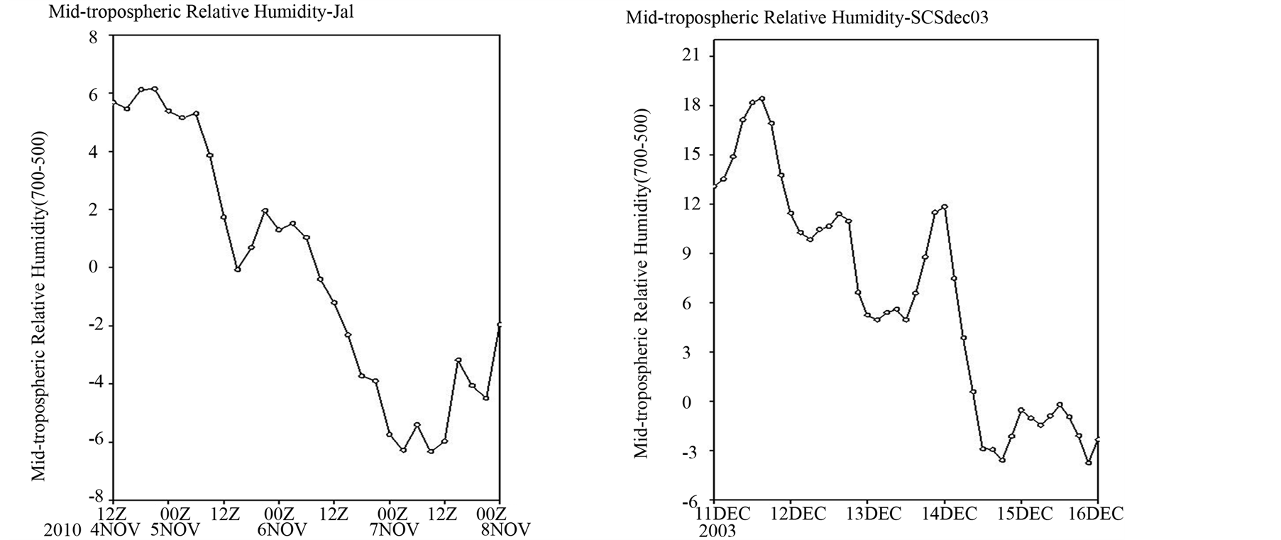 (b)
(b)
Figure 5. Time evolution mid-tropospheric relative humidity calculated at the relative humidity difference between 700 hPa and 500 hPa level, averaged over corresponding cyclone path for a) Laila; b) Aila; c) Jal; d) SCS.
4.3.2. Mid-Tropospheric Parameters Affecting Cyclone Intensity
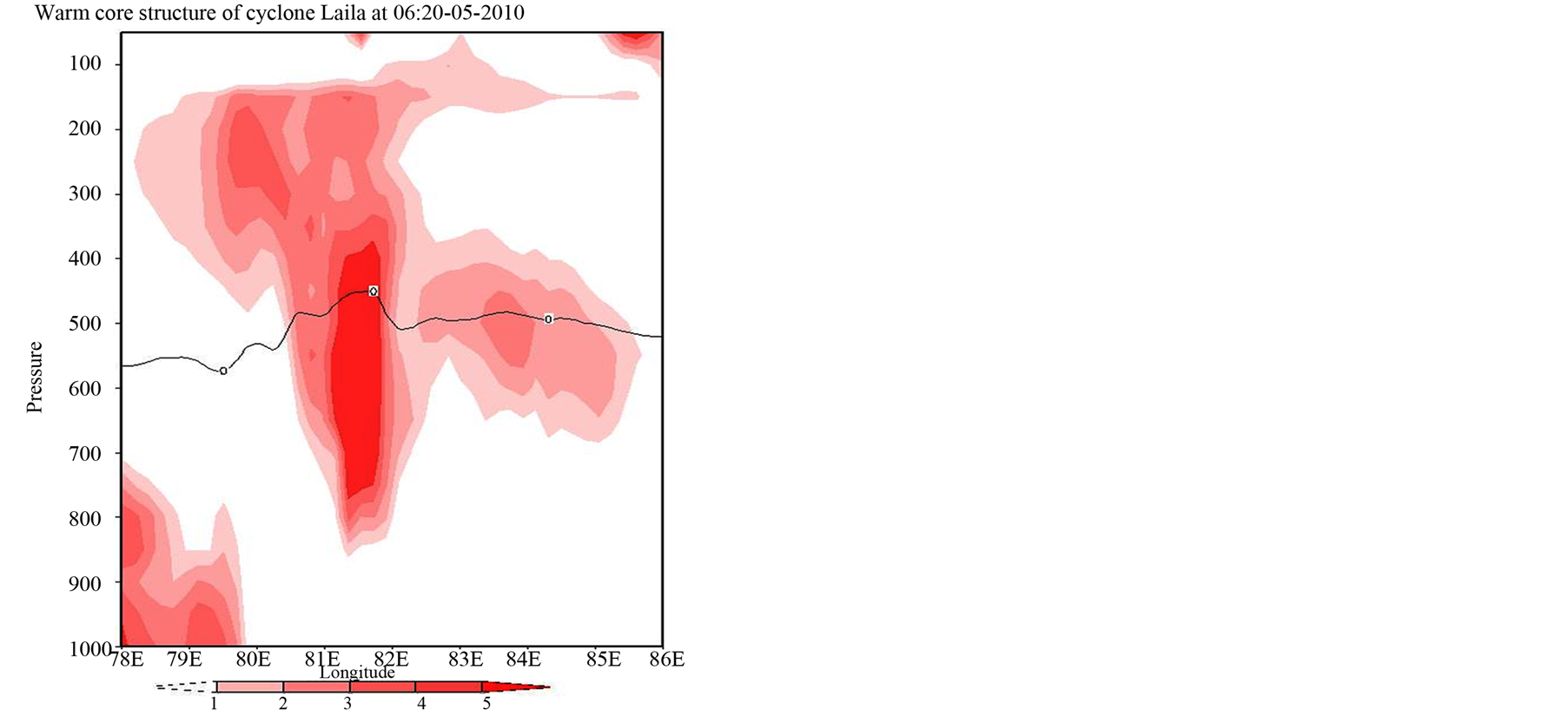
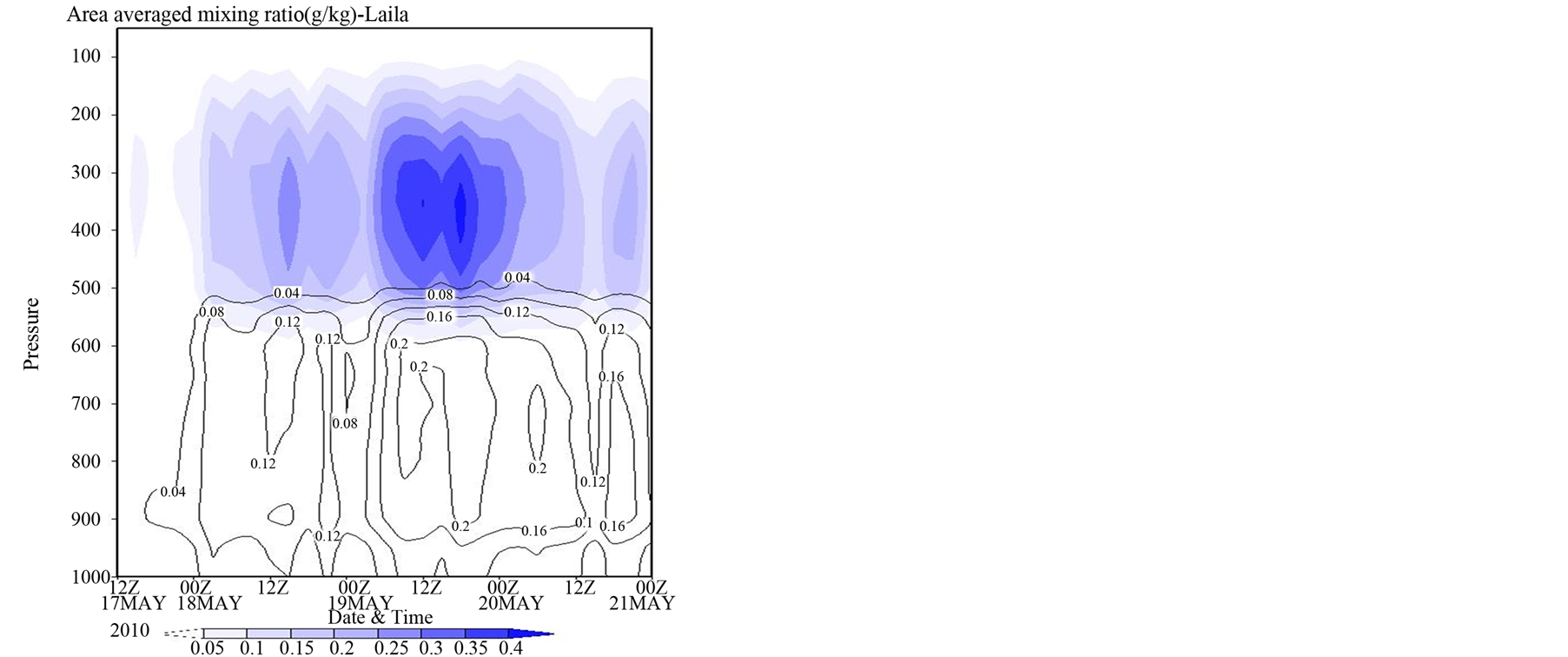
The warm core structure at the mature stage of the respective cyclones is shown in the Figure 6. The primary warming maxima with magnitudes of 4˚C - 5˚C lies in the mid-troposphere while the secondary warming maxima lies in the upper troposphere for all cyclones. The increased warming in the mid-troposphere can also be demonstrated by plotting time evolution of the mid-tropospheric temperature gradient i.e. temperature difference between 850 hPa and 500 hPa in ˚C (figure not shown). For all the four cyclones the temperature gradient values at the initial stage are more than 20˚C, and then the values oscillate during the developing stage of cyclone and thereafter decrease continuously till landfall. This means that there is warming in the middle troposphere which causes decrease in the lower and mid-level temperature difference. To explore the reason behind the mid-tropospheric warming, time evolution of area averaged mixing ratio for all the cyclones is plotted (Figure 7). The shaded region is the frozen hydrometeors which include ice, snow and graupel and contour are drawn for the liquid hydrometeors like rain and cloud water. For pre-monsoon cyclones, total hydrometeor concentration peak (Frozen and liquid) is clearly seen 12 hrs before the mature stage but for post-monsoon cyclones, the peak is observed at least 36 hrs prior to the mature stage of the cyclones. Increase in the frozen hydrometeors concentration contributes to more release of latent heat of freezing (Lord et al. [34] , Mukhopadhyay et al. [16] , Deshpande et al. [7] ), which in turn causes maximum heating in the midtroposphere and thus causes the warm core structure of cyclone which is observed in all the preand post-monsoon cases of weak cyclonic storms. The
 (a)
(a)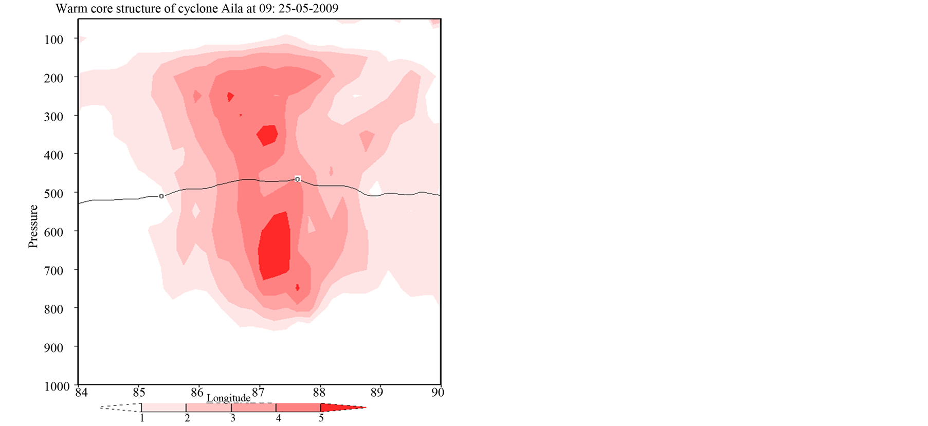 (b)
(b)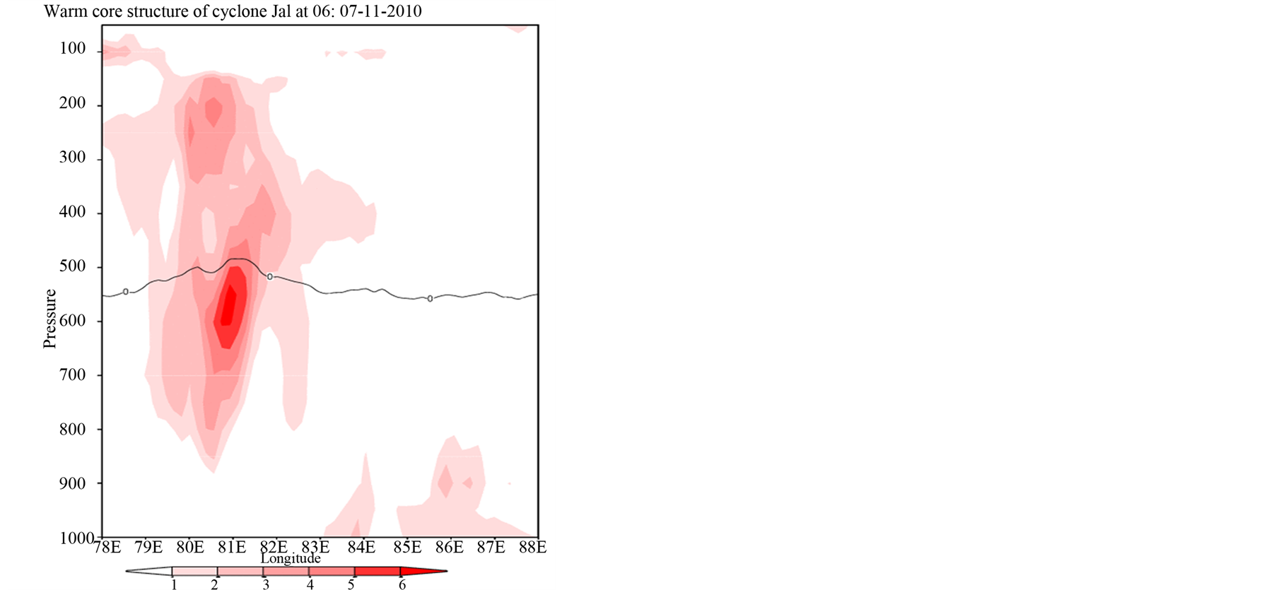 (c)
(c)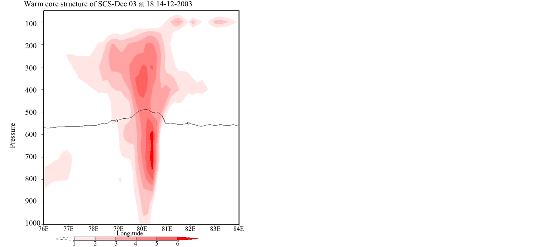 (d)
(d)
Figure 6. Warm core (˚C) structure of cyclone a) Laila at 06:20-05-2010; b) Aila at 09:25-05-2010; c) Jal at 06:07-11-2010; d) CS at 18:14-12-2010.
comparison between the peaks in the relative humidity plot (Figure 5) and higher values in the area averaged mixing ratio (Figure 7) shows that high concentration of frozen hydrometeors corresponds to the increase in relative humidity at 500 hPa level and higher values of the liquid hydrometeors corresponds to the increased relative humidity values at 700 hPa level.
Thus the representation of boundary layer processes along with the mid-tropospheric processes i.e. both may contribute towards the cyclone intensity.
4.4. Rainfall
Left panel of Figure 8 shows 24 hours accumulated TRMM rainfall (cm) at the observed landfall and right panel shows the model simulated 24 hrs accumulated rainfall (cm) at the model landfall for four cyclones: Laila, Aila, Jal and SCS. The rainfall is overestimated by the model for all the cyclones except for SCS case. For cyclone Laila, as the simulated landfall location is slightly to the north of the observed landfall, the rainfall maxima is also simulated to the north of the observed TRMM rainfall maxima. The model simulated rainfall is slightly
 (a)
(a)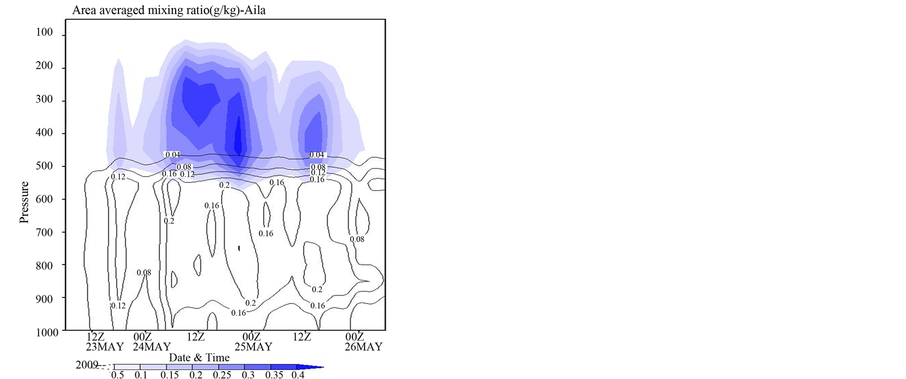 (b)
(b)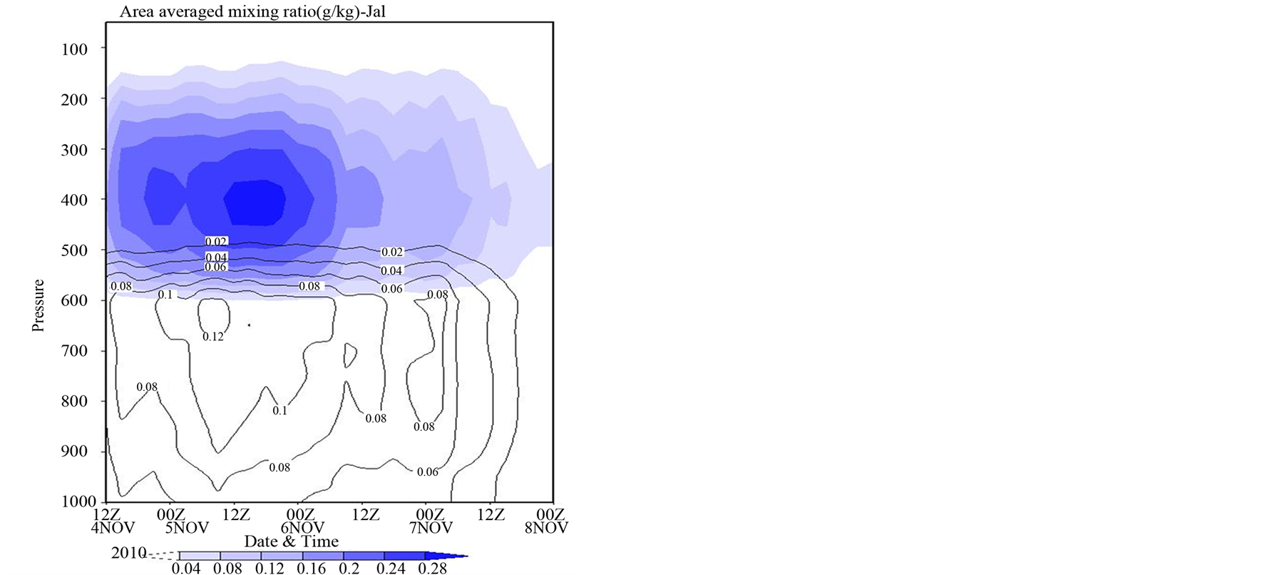 (c)
(c)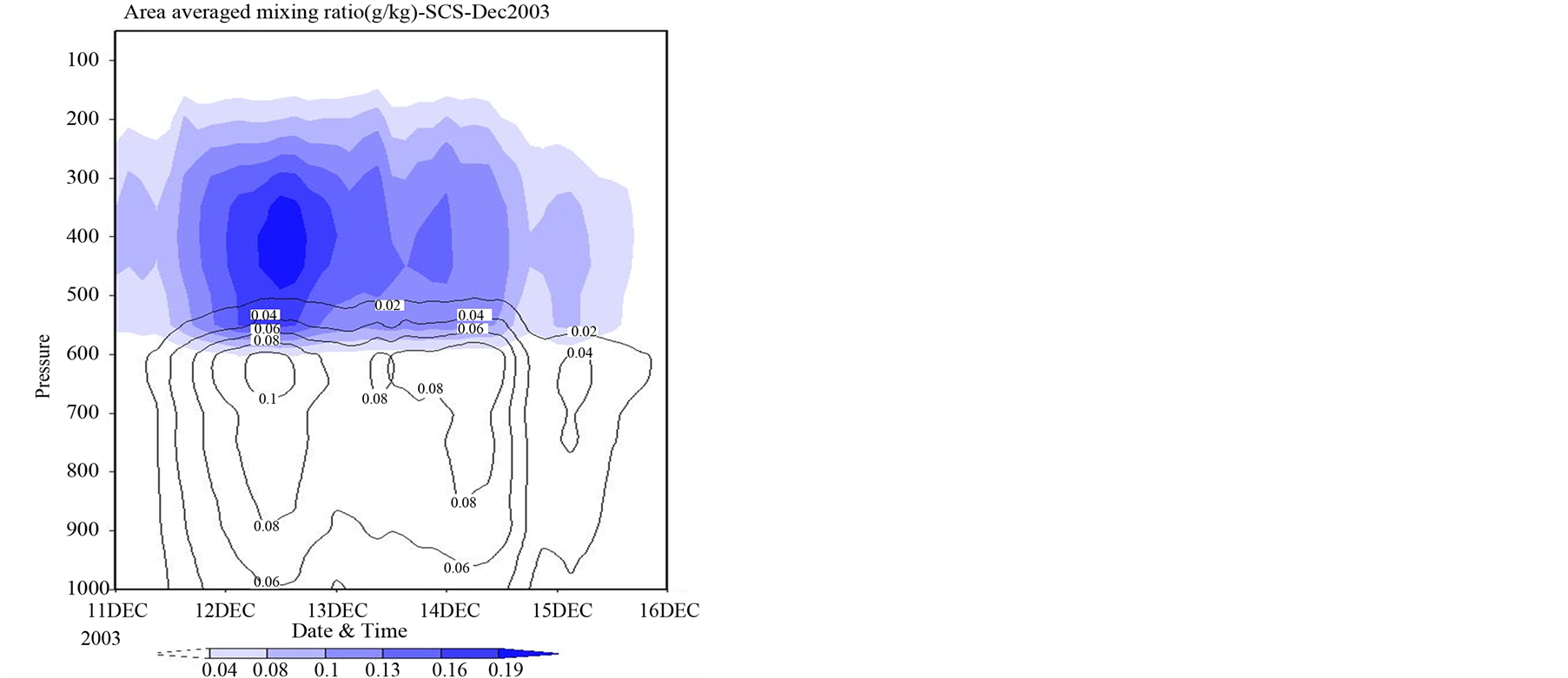 (d)
(d)
Figure 7. Time evolution of Area averaged mixing ratio (g/kg) averaged over cyclone path for a) Laila; b) Aila; c) Jal; d) SCS.
overestimated with the magnitudes greater than 40 cm whereas the observed rainfall values are less than 40 cm. In case of Aila and Jal cyclone, TRMM rainfall lies in the range 10 to 30 cm whereas the model simulated values are more than 30 cm at the corresponding landfall location. For SCS cyclone, the TRMM rainfall maximum is observed on the ocean itself. The model simulated rainfall maxima follows the track simulated by the model.
5. Conclusions
Weak cyclones due to their slow motion and quasi-stationary nature cause very heavy rainfall and in turn large amount of damage to the property and hence it is very important to study these cyclones. Four such cyclones viz, Laila, Aila, Jal and SCS are studied by keeping BMJ-YSU-WSM6 combination of different physical parameterization schemes fixed in WRF-ARW model. The main findings of the study are:
The surface track, landfall time and landfall position are well simulated by BMJ-YSU-WSM6 combination of physical processes for all cases of cyclones except for SCS. It may be because of the model and thus the BMJ scheme is able to simulate proper upper level steering flow which drives the cyclone to move in the same direction as that of steering current. For weak storms which are quasi-stationary in nature, BMJ may be able to produce proper large scale environmental flow and thus the track of all cyclones except SCS.
The intensity is overestimated in all the cases irrespective of preand post-monsoon cyclones. To understand
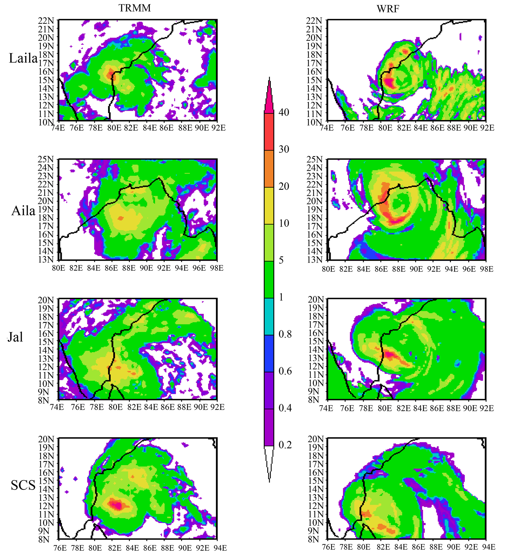
Figure 8. 24 hrs averaged rainfall in cm at the landfall time for four cyclones viz Laila, Aila, Jal, SCS. left panel: TRMM Rainfall and right panel: WRF model simulated rainfall.
the reason behind the overestimation, we studied mature stage structure of cyclones and also time evolution of lower-tropospheric and mid-tropospheric factors affecting the cyclone intensity. Boundary layer processes and deep mixing in and above the PBL top assumed in the YSU PBL scheme are explained by increase in the mid-tropospheric (500 hPa) humidity upto mature stage of the cyclones. Increase in the mid-tropospheric humidity causes higher production of the frozen hydrometeors and thus large amount of latent heat release, which in turn causes higher intensity of the cyclone. Similar conclusions have been found by Lord et al. [34] as well as Lord and Lord [35] in their study. The rainfall is overestimated by the model for all the cyclones (except for SCS) and is consistent with the intensity overestimation by model.
Careful examination of genesis location for all cyclones indicated that the cyclones Laila, Jal and Aila have the genesis location away from the equatorial belt (~8˚N for Jal cyclone, ~11˚N for Laila and ~17˚N for Aila), but for SCS, the genesis location is relatively close to the equator (~4˚N). We feel that for SCS, in addition to the improper upper level steering flow, the cross equatorial flow and hence, equatorial dynamics has some role in determining the track of SCS. Thus proper representation of equatorial dynamics in the parameterization schemes and thus in the model may lead to the accurate simulation of the cyclones having genesis near the equatorial belt. We plan to work in detail for cyclones which have genesis very close to equator (~3˚N).
Acknowledgements
The authors wish to thank the Director, Indian Institute of Tropical Meteorology (IITM), Pune for his encouragement and support. Authors acknowledge the use of WRF-ARW model, which is made available on the Internet by the Mesoscale and Microscale division of NCAR. The use of NCEP-FNL data, RTG-SST data, IMD observations and GrADS software is acknowledged with thanks.
References
- Charney, J.G. and Eliassen, A. (1964) On the Growth of the Hurricane Depression. Journal of the Atmospheric Sciences, 21, 68-75.
http://dx.doi.org/10.1175/1520-0469(1964)021<0068:OTGOTH>2.0.CO;2 - Gray, W.M. (1968) Global View of the Origin of Tropical Disturbances and Storms. Monthly Weather Review, 96, 669-700. http://dx.doi.org/10.1175/1520-0493(1968)096<0669:GVOTOO>2.0.CO;2
- Holland, G.J. and Merill, R.T. (1984) On the Dynamics of Tropical Cyclone Structural Changes. Quarterly Journal of the Royal Meteorological Society, 110, 723-745.
http://dx.doi.org/10.1002/qj.49711046510 - Craig, G.C. and Gray, S.L. (1996) CISK or WISHE as the Mechanism for Tropical Cyclone Intensification. Journal of the Atmospheric Sciences, 53, 3528-3540. http://dx.doi.org/10.1175/1520-0469(1996)053<3528:COWATM>2.0.CO;2
- Holland, G.J. (1983) Tropical Cyclone Motion: Environmental Interaction plus a Beta Effect. Journal of the Atmospheric Sciences, 40, 328-342.
http://dx.doi.org/10.1175/1520-0469(1983)040<0328:TCMEIP>2.0.CO;2 - Pattanayak S. and Mohanty, U.C. (2008) A Comparative Study on Performance of MM5 and WRF Models in Simulation of Tropical Cyclones over Indian Seas. Current Science, 95, 923-936.
- Deshpande, M., Pattanaik, S. and Salvekar, P.S. (2010) Impact of Physical Parameterization Schemes on Numerical Simulation of Super Cyclone Gonu. Natural Hazards, 55, 211-231.
http://dx.doi.org/10.1007/s11069-010-9521-x - Deshpande, M., Pattnaik, S. and Salvekar, P.S. (2012) Impact of Cloud Parameterization on the Numerical Simulation of a Super Cyclone. Annales Geophysicae, 30, 775-795.
http://dx.doi.org/10.5194/angeo-30-775-2012 - Trivedi, D.K., Mukhopadhyay, P. and Vaidya, S.S. (2006) Impact of Physical Parameterization Schemes on the Numerical Simulation of Orissa Super Cyclone (1999). Mausam, 57, 97-110.
- Osuri, K.K., Mohanty, U.C., Routray, A., Kulkarni, M.A. and Mohapatra, M. (2012) Customization of WRF-ARW Model with Physical Parameterization Schemes for the Simulation of Tropical Cyclones over North Indian Ocean. Natural Hazards, 63, 1337-1359. http://dx.doi.org/10.1007/s11069-011-9862-0
- Osuri, K.K., Mohanty, U.C., Routray, A., Mohapatra, M. and Nivogi, D. (2013) Real-Time Track Prediction of Tropical Cyclones over the North Indian Ocean Using the ARW Model. Journal of Applied Meteorology and Climatology, 52, 2476-2492. http://dx.doi.org/10.1175/JAMC-D-12-0313.1
- Rao, D.V.B., Prasad, D.H. and Srinivas, D. (2009) Impact of Horizontal Resolution and the Advantages of the Nested Domains Approach in the Prediction of Tropical Cyclone Intensification and Movement. Journal of Geophysical Research: Atmospheres, 114, Published Online.
- Srinivas, C.V., Venkatesan, R., Rao, D.V.B. and Prasad, D.H. (2007) Numerical Simulation of Andhra Severe Cyclone (2003) Model Sensitivity to Boundary Layer and Convection Parameterization. Pure and Applied Geophysics, 164, 1-23. http://dx.doi.org/10.1007/s00024-007-0228-1
- Srinivas, V., Venkatesan, R., Yesubabu, V. and Ramarkrishna, S.S.V.S. (2010) Impact of Assimilation of Conventional and Satellite Meteorological Observations on the Numerical Simulation of a Bay of Bengal Tropical Cyclone of Nov 2008 near Tamilnadu Using WRF Model. Meteorology and Atmospheric Physics, 110, 19-44. http://dx.doi.org/10.1007/s00703-010-0102-z
- Raju, P.V.S., Potty, J. and Mohanty, U.C. (2011) Sensitivity of Physical Parameterizations on the Prediction of Tropical Cyclone Nargis over the Bay of Bengal Using WRF Model. Meteorology and Atmospheric Physics, 113, 125-137. http://dx.doi.org/10.1007/s00703-011-0151-y
- Mukhopadhyay, P., Taraphdar, S. and Goswami, B.N. (2011) Influence of Moist Processes on Track and Intensity Forecast of Cyclones over the Indian Ocean. Journal of Geophysical Research: Atmospheres, 116, Published Online. http://dx.doi.org/10.1029/2010JD014700
- Srinivas, C.V., Rao, D.V.B., Yesubabu, V., Baskarana, R. and Venkatraman, B. (2013) Tropical Cyclone Predictions over the Bay of Bengal Using the High-Resolution Advanced Research Weather Research and Forecasting (ARW) Model. Quarterly Journal of the Royal Meteorological Society, 139, 1810-1825. http://dx.doi.org/10.1002/qj.2064
- Li, X. and Pu, Z. (2008) Sensitivity of Numerical Simulation of Early Rapid Intensification of Hurricane Emily (2005) to Cloud Microphysical and Planetary Boundary Layer Parameterizations. Monthly Weather Review, 136, 4819-4838. http://dx.doi.org/10.1175/2008MWR2366.1
- Efstathiou, G.A., Zoumakis, N.M., Melas, D. and Kassomenos, P. (2012) Impact of Precipitating Ice on the Simulation of a Heavy Rainfall Event with Advanced Research WRF Using Two Bulk Microphysical Schemes. Asia-Pacific Journal of Atmospheric Sciences, 48, 357-368.
http://dx.doi.org/10.1007/s13143-012-0034-2 - Tao, W., Shi, J.J., Chen, S.S., Lang, S., Lin, P., Hong, S.Y., Peters-Lidard, C. and Hou, A. (2011) The Impact of Microphysical Schemes on Hurricane Intensity and Track. Asia-Pacific Journal of Atmospheric Sciences, 47, 1-16. http://dx.doi.org/10.1007/s13143-011-1001-z
- Kanase, R.D. and Salvekar, P.S. (2011) Numerical Simulation of Severe Cyclonic Storm LAILA (2010): Sensitivity to Initial and Cumulus Parameterization Schemes. Proceedings of Disaster Risk Vulnerability Conference, 1, 165-170.
- Skamarock, W.C., Klemp, J.B., Dudhia, J., Gil, D.O., Barker, D.M., Duda, M.G., Huang, X.Y., Wang, W. and Powers, J.G. (2008) A Description of the Advanced Research WRF Version 3 NCAR Tech. Note NCAR/TN-4751 STR, 1-113. http://www.mmm.ucar.edu/wrf/users/docs/arw_v3_bw.pdf
- Betts, A.K. (1986) A New Convective Adjustment Scheme Part I: Observational and Theoretical Basis. Quarterly Journal of the Royal Meteorological Society, 112, Article ID: 677691.
- Betts, A.K. and Miller, M.J. (1986) A New Convective Adjustment Scheme Part II: Single Column Tests Using GATE Wave, BOMEX, and Arctic Air Mass Data Sets. Quarterly Journal of the Royal Meteorological Society, 112, 693-709.
- Janjic, Z.I. (1994) The Step-Mountain Eta Coordinate Model: Further Developments of the Convection, Viscous Sublayer, and Turbulence Closure Schemes. Monthly Weather Review, 122, 927-945. http://dx.doi.org/10.1175/1520-0493(1994)122<0927:TSMECM>2.0.CO;2
- Hong, S.Y., Dudhia, J. and Chen, S.H. (2004) A Revised Approach to Ice Microphysical Processes for the Bulk Parameterization of Cloud and Precipitations. Monthly Weather Review, 132, 103-120. http://dx.doi.org/10.1175/1520-0493(2004)132<0103:ARATIM>2.0.CO;2
- Houze, R.A., Hobbs Jr., P.V., Herzegh, P.H. and Parsons, D.B. (1979) Size Distributions of Precipitation Particles in Frontal Clouds. Journal of the Atmospheric Sciences, 36, 156-162.
http://dx.doi.org/10.1175/1520-0469(1979)036<0156:SDOPPI>2.0.CO;2 - Tripoli, G.J. and Cotton, W.R. (1980) A Numerical Investigation of Several Factors Contributing to the Observed Variable Intensity of Deep Convection over South Florida. Journal of Applied Meteorology, 19, 1037-1063. http://dx.doi.org/10.1175/1520-0450(1980)019<1037:ANIOSF>2.0.CO;2
- Hong, S.Y. and Pan, H.L. (1996) Nonlocal Boundary Layer Vertical Diffusion in a Medium-Range Forecast Model. Monthly Weather Review, 124, 2322-2339. http://dx.doi.org/10.1175/1520-0493(1996)124<2322:NBLVDI>2.0.CO;2
- Hong, S.Y. and Lim, J.O.J. (2006) The WRF Single Moment 6 Class Microphysics Scheme (WSM6). Journal of the Korean Meteorological Society, 42, 129-151.
- RSMC Report (2010) A Report on Cyclonic Disturbances over North Indian Ocean during 2009. India Meteorological Department, New Delhi.
- RSMC Report (2009) A Report on Cyclonic Disturbances over North Indian Ocean during 2003. India Meteorological Department, New Delhi.
- RSMC Report (2004) A Report on Cyclonic Disturbances over North Indian Ocean during 2010. India Meteorological Department, New Delhi.
- Lord, S.J., Willoughby, H.E. and Piotrowicz, J.M. (1984) Role of a Parameterized Ice-Phase Microphysics in an Axisymmetric, Nonhydrostatic Tropical Cyclone Model. Journal of the Atmospheric Sciences, 41, 2836-2848. http://dx.doi.org/10.1175/1520-0469(1984)041<2836:ROAPIP>2.0.CO;2
- Lord, S.J. and Lord, J.M. (1988) Vertical Velocity Structure in an Axisymmetric, Nonhydrostatic Tropical Cyclone Model. Journal of the Atmospheric Sciences, 45, 1453-1461. http://dx.doi.org/10.1175/1520-0469(1988)045<1453:VVSIAA>2.0.CO;2