International Journal of Astronomy and Astrophysics
Vol.06 No.03(2016), Article ID:70238,4 pages
10.4236/ijaa.2016.63022
Modelling and Analysis of the Hubble Diagram of 280 Type SNIa Supernovae and Gamma Ray Bursts Redshifts with Analytical and Empirical Redshift/Magnitude Functions
Laszlo A. Marosi
67061 Ludwigshafen am Rhein, Germany

Copyright © 2016 by author and Scientific Research Publishing Inc.
This work is licensed under the Creative Commons Attribution International License (CC BY).
http://creativecommons.org/licenses/by/4.0/


Received 20 July 2016; accepted 28 August 2016; published 31 August 2016
ABSTRACT
Based on an analysis of 280 Type SNIa supernovae and gamma-ray bursts redshifts in the range of z = 0.0104 - 8.1 the Hubble diagram is shown to follow a strictly exponential slope predicting an exponentially expanding or static universe. At redshifts > 2 - 3 ΛCDM models show a poor agreement with the observed data. Based on the results presented in this paper, the Hubble diagram test does not necessarily support the idea of expansion according to the big-bang concordance model.
Keywords:
Magnitude, Redshift Data Fitting, Supernovae, Gamma Ray Bursts, Hubble Diagram, ΛCDM Cosmological Model

1. Introduction
Based on an analysis of 280 Type SNIa supernovae and gamma ray bursts redshift (z) data Marosi [1] has shown that the best-fit function to represent the observational z/extinction-corrected distance moduli (μ) data set is the exponential equation μ = 44.109769 × z0.059883. Recently, a number of papers have appeared proposing different analytical formulae for describing the experimental z/μ relationship: Sorrell [2] , Vigoureux, Vigoureux and Langlois [3] Traunmüller [4] and Churoux [5] . In this paper, observed z/μ data of 280 Type SNIa supernovae and gamma ray bursts in the range of z = 0.0104 - 8.1 are compared to results calculated on the basis of these theoretically derived and empirical functions and the Lambda cold dark matter (ΛCDM) model. The aim of this paper is to examine which of the above functions and models fits the observations more accurately. We expect that in the high RS range it should be possible to decide whether the Hubble diagram follows the distance/z relationship as predicted by the ΛCDM model, or the exponential tired light formula.
2. Data Collection and Processing
The z/μ data set consists of 171 gold-set data, Riess et al. [6] , and 109 cosmology independent calibrated gamma-ray bursts (GRB) data consisting of 59 high-RS data (Hymnium data set) and 50 low RS GRBs obtained by Wei [7] from the 557 Union 2-compilation.
The following mathematical functions and cosmological models were used to perform a global fitting over the RS range of z = 0.0104 - 8.1.
 (Marosi, 2014) (1)
 (Vigoureux et al., 2014) (2)
 (Churoux, 2015) (3)
ΛCDM model with ,
,  ,
,  and
and  (4)
(4)
ΛCDM model with ,
,  ,
,  and
and  (5)
(5)
The μ values on basis of the ΛCDM models were calculated using:
 (6)
(6)
where DL (Pc) is the luminosity distance. The luminosity distances were calculated using the cosmological calculator described by Wright [8] .
For preparing the linear tS/z Hubble diagram, using Equation (7) the fitted z/μ data were converted into the corresponding tS/z datasets.
The photon flight-time tS was calculated using:
 (7)
(7)
In Equation (7) tS means the flight time of the photons (sec.) from the co-moving radial distance DC to the observer, tS = DC/c, which is proportional to the DC (Pc) that goes into the linear Hubble law.
In order to complete the fitted z/μ data set in the high RS range of tS × 10−14 = 6000 - 11000, in addition to the measured RSs, using Equation (2), 41 equidistant tS/z data points were included into the Hubble diagram. The addition of the 41 additional data points is necessary to perform the ∑χ2-test between the best fit and the ΛCDM models because only few observations are available in this redshift range. The tS/RS values were calculated on the basis of Functions (2) and (5).
Excel and Excel Solver were used for data fitting, refinement, and data presentation.
3. Results
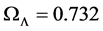
Figure 1 shows results of the z/μ data fitting with Functions (1)-(5).
It is easy to see by visual examination of Figure 1 that there are only minor differences between the fit curves calculated with Functions (1) and (2), whilst the ΛCDM model with H0 = 72.6 km s−1 Mpc−1 (bottom line in Figure 1) is slightly but perceptibly different.
The most reliable measure to quantify the differences between the individual fit curves turned out to be the ∑χ2-test. The goodness of fit indicators are shown in Table 1.
The ∑χ2-test obviously favors the trend-lines obtained with Functions (1) and (2) and these two curves are practically congruent. On basis of the data presented in Table 1 the analytical best-fit Function (2) will be used as the best representation of the observed z/μ data in the following discussion.
Figure 2(a) and Figure 2(b) show Hubble diagrams calculated on basis of the Functions (2), (4) and (5).
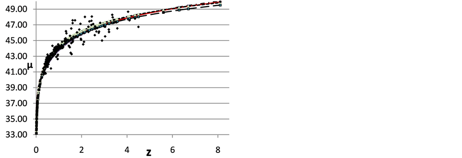
Figure 1. Squares: observed z/μ data; long dash-dot line: (2); solid line: (1); dash-dot line: (3); long dashed line; ΛCDM, H0 = 72.6 km s−1 Mpc−1; short dashed line: ΛCDM, H0 = 62.5 km s−1 Mpc−1.

Table 1. Goodness of fit indicators of the z/μ data trend-lines.
 (a) (b)
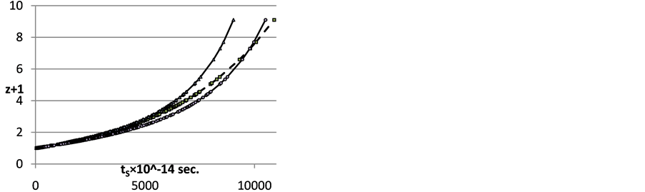
Figure 2. (a) Redshift of type Ia supernovae as a function of tS = DC/c. Squares (dashed line): tS/z data inferred from the potential best-fit curve of the observed z/μ diagram. Triangles: tS/z relationship derived from the ΛCDM model with H0 = 72.6 km s−1 Mpc−1, Circles: tS/z relationship derived from the ΛCDM model with H0 = 62.5 km s−1 Mpc−1; (b) squares: tS/z data inferred from the potential best-fit curve of the observed z/μ diagram, solid line: exponential trend-line (Excel).
4. Discussion
The most important result of the Hubble diagram test is that fitting the tS/z data with Function (2) and H0 = 62.5 km s−1 Mpc−1 (dashed line in Figure 2(a)) leads exactly to the exponential function:
 (8)
(8)
as illustrated in Figure 2(b).
In spite of numerous correction factors and unknown constituents, dark matter (DM) and dark energy (DE), the ΛCDM models show a poor agreement with the observed data: as shown in Figure 2(a) the ΛCDM model with H0 = 62.5 km s−1 Mpc−1 departs from the best-fit curve for z + 1 < 6.5 to the bottom, for z + 1 > 6.5 to the upper side of the trend-line. The deviations are of a systematic (nonstatistical) nature and, therefore, the model cannot reflect the observational exponential slope.
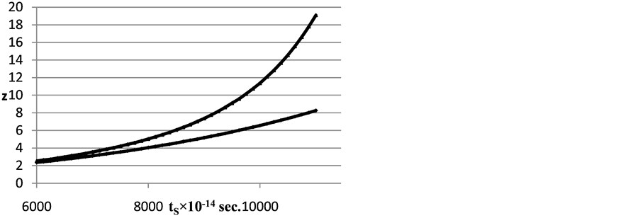
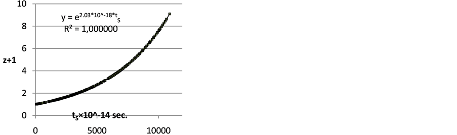
Figure 3. Bottom line: Calculated data points from the best-fit Function (2); upper line: calculated data points for the tS/z relationship derived from the ΛCDM model with H0 = 72.6 km s−1 Mpc−1. From [1] .
In the range of z > 3 the ΛCDM model with H0 = 72.6 km s−1 Mpc−1 shows a sharp increase in slope and departs considerably from the observed exponential function. For performing the ∑χ2-test in the high RS range of tS × 10−14 = 6000 - 11000 (Figure 3), using Equation (2), 41 calculated tS/z data points were included into the Hubble diagram. The ∑χ2-test leads to a statistical significance between the observed tS/μ and the calculated ΛCDM data of P = 0.053, indicating that from the statistical point of view, the two models are essentially different.
5. Conclusions
The results presented in this paper have demonstrated that the ΛCDM-model cannot fit the strictly exponential slope of the Hubble diagram in the entire RS range of z = 0.0104 - 8.1, showing that the underlying theory is, at best, incomplete. A reconsideration of the ΛCDM-model appears warranted.
The Hubble diagram test leads to the significant conclusion that either: (1) the universe expanded exponentially during the whole time of its expansion history (at least in the range of z = 0.0104 - 8.1); or (2) the universe is static and the RS of spectral lines is caused by some as-yet unidentified mechanism. However, both of these models, the exponentially expanding and the static universe models have their own crucial problems; the discussion of them is not within the scope of this paper.
Cite this paper
Laszlo A. Marosi, (2016) Modelling and Analysis of the Hubble Diagram of 280 Type SNIa Supernovae and Gamma Ray Bursts Redshifts with Analytical and Empirical Redshift/Magnitude Functions. International Journal of Astronomy and Astrophysics,06,272-275. doi: 10.4236/ijaa.2016.63022
References
- 1. Marosi, L.A. (2014) Hubble Diagram Test of 280 Supernovae Redshift Data. Journal of Modern Physics, 5, 29-33.
http://dx.doi.org/10.4236/jmp.2014.51005 - 2. Sorrell, W.H. (2009) Misconceptions about the Hubble Recession Law. Astrophysics and Space Science, 323, 205-211.
http://dx.doi.org/10.1007/s10509-009-0057-z - 3. Vigoureux, J.M., Vigoureux, B. and Langlois, M. (2014) An Analytical Expression for the Hubble Diagram of Supernovae and Gamma-Ray Bursts. arXiv:1411.3648v1.
- 4. Traunmüller, H. (2014) From Magnitudes and Redshifts of Supernovae, Their Light-Curves, and Angular Sizes of Galaxies to a Tenable Cosmology. Astrophysics and Space Science, 350, 755-767.
http://dx.doi.org/10.1007/s10509-013-1764-z - 5. Churoux, P. (2015) A New Interpretation of the Hubble Law. Journal of Modern Physics, 6, 1227-1232.
http://dx.doi.org/10.4236/jmp.2015.69127 - 6. Riess, A.G., Sirolger, A.G., Tonry, J., et al. (2004) Type Ia Supernova Discoveries at z > 1 from the Hubble Space Telescope: Evidence for Past Deceleration and Constraints on Dark Energy Evolution. The Astrophysical Journal, 602, 665-687.
http://dx.doi.org/10.1086/383612 - 7. Wei, H. (2010) Observational Constraints on Cosmological Models with the Updated Long Gamma-Ray Bursts. Journal of Cosmology and Astroparticle Physics, 2010, Article ID: 020.
http://dx.doi.org/10.1088/1475-7516/2010/08/020 - 8. Wright, E.L. (2006) Cosmological Calculator. PASP, 188, 1711-1715, Last Modified 06-12-2014.