International Journal of Astronomy and Astrophysics
Vol. 2 No. 1 (2012) , Article ID: 18178 , 9 pages DOI:10.4236/ijaa.2012.21005
Large-Eddy Simulation of the Three-Dimensional Experiment on Richtmyer-Meshkov Instability Induced Turbulence
1Institute of Fluid Physics, China Academy of Engineering Physics, Mianyang, China
2National Key Laboratory of Shock Wave and Detonation Physics, Institute of Fluid Physics, China Academy of Engineering Physics, Mianyang, China
Email: *bjsong@foxmail.com
Received January 9, 2012; revised February 12, 2012; accepted February 22, 2012
Keywords: MVFT3D; Large Eddy Simulation; SGS; Interface Instability; Turbulence Mixing
ABSTRACT
A program MVFT3D of large-eddy simulation is developed and performed to solve the multi compressible NavierStokes equations. The SGS dissipation and molecular viscosity dissipation have been analyzed, and the former is much larger than the later. Our test shows that the SGS dissipation of Vreman model is smaller than the Smagorinsky model. We mainly simulate the experiment of fluid instability of shock-accelerated interface by Poggi in this paper. The decay of the turbulent kinetic energy before the first reflected shock wave-mixing zone interaction and its strong enhancement by re-shocks are presented in our numerical simulations. The computational mixing zone width under double re-shock agreement well with the experiment, and the decaying law of the turbulent kinetic energy is consistent with Mohamed and Larue’s investigation. Also, by using MVFT3D we give some simulation results of the inverse Chevron model from AWE. The numerical simulations presented in this paper allow us to characterize and better understand the Richtmyer-Meshkov instability induced turbulence, and the code MVFT3D is validated.
1. Introduction
An instability induced by a shock wave colliding with an interface between two materials of different density is known as the Richtmyer-Meshkov (RM) instability. When two different fluids are impulsively accelerated into each other by a shock wave, small perturbations at the interface grow first linearly and then evolve into nonlinear structures formed of “bubbles” and “spikes”. Afterwards, it may lead to the formation of a turbulent mixing zone (TMZ). The shock wave interaction with a TMZ has gained much attention over the past decades, due to its important in physics systems such as inertial confinement fusion (ICF) and astrophysical phenomena [1,2]. A professional international workshop on the physics of compressible turbulent mixing (IWPCTM) performed every two years. These workshop are mainly devoted to the problems of hydrodynamic instabilities of different density fluid interfaces submitted either to a constant or varying acceleration (Rayleigh-Taylor instability, RT) or to an impulsive acceleration generated by a shock wave (Richtmyer-Meshkov instability, RM). These instabilities are studied at all stages, that is from the development of the initial small perturbation (linear phase) to the end of the process (turbulent mixing phase) [3-5]. Shock-tube experiments have been performed to study the shock induced turbulent mixing at SF6-air interface by Poggi [6]. In their experiments, instantaneous velocities in a gaseous mixture arising from the shock-wave-induced RM instability are measured by Laser Doppler Anemometry (LDA). These experiments give a direct measurement of turbulence for the first time [7]. These shock-tube experiments of SF6 incident on air demonstrate that the initial small-scale perturbations of the interface develop into a turbulent mixing zone, whose turbulence level decays before the first reflected shock wave arriving from the end wall. Afterwards, the reshock interaction amplifies the turbulence level through a baroclinic effect. Recently, author investigated the interface instability of nonuniform flow initial conditions [8] and evolution of elliptic heavy SF6 gas cylinder sourround by air when accelerated by a planar Mach a.15 shock [9], and well conducted the experiment and numerical simulations.
In this paper, based on the multi-viscous-fluid piecewise parabolic method [10], the Vreman [11] and Smagorinsky [12] subgrid eddy viscosity models are employed to solve the Navier-Stokes equations. A three-dimensional large eddy simulation (LES) code MVFT3D (3D multiviscous-fluid and turbulence) for the multi-viscosity-fluid and turbulence from the fluid interface instability is developed. The SGS dissipation and molecular viscosity dissipation have been analyzed by the simulation of AWE’s shuck tube [13] RM instability experiment. We mainly simulate the experiment of fluid instability of shock-accelerated interface by Poggi in this paper. Experiment shows that a turbulent mixing zone is generated by the incident shock wave. We can see in numerical simulations the decay of the turbulent kinetic energy before the first reflected shock wave-mixing zone interaction and its strong enhancement by re-shocks. The computational mixing zone width under double re-shock agreement well with the experiment, and the decaying law of the turbulent kinetic energy is consistent with Mohamed and Larue’s investigation. By the numerical simulations, we compare the factors that affect the mixing zone width, which include the Smagorinsky model and the Vreman SGS model, as well as the three kinds of random wavelength ranges. We focus on the three dimensional simulation of shock induced turbulence. The goal of our simulation is to perform highly resolved three-dimensional numerical simulations of flows subsequent to the RM instability, and study both the transitional and the turbulent regimes. In the last part of the paper, we give some simulation results of the inverse Chevron model from AWE. However, because there is no definite experimental data in the literature [14], we have no quantitative comparison. After all, through quantitative and qualitative comparison with experiment, the method and code of MVFT3D is validated and can be used to investigate the problem of RM instability induced turbulence.
2. Numerical Method
2.1. Governing Equations
LES [15,16] is an intermediate approach between DNS (direct numerical simulation) and RANS (Reynolds-averaging equations), capable of simulating flow features such as significant flow unsteadiness and strong vortexacoustic couplings, with respect to accuracy and computational cost. This approach is based on the multi-viscous-fluid piecewise parabolic method, [10] and tries to solve filtered Navier-Stokes equations closed with a Vreman subgrid model for turbulence stress tensor. The equations have the flowing forms:
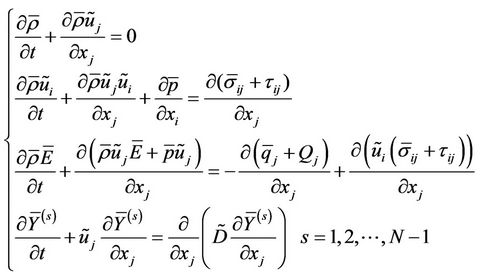 (1)
(1)
![]() is the viscous stress tensor,
is the viscous stress tensor, ![]() is the subgrdiscale (SGS) stress tensor,
is the subgrdiscale (SGS) stress tensor, ![]() is the energy flux of a unit time and space,
is the energy flux of a unit time and space, 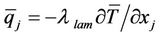 ,
, ![]() ,
, ![]() ,
, ![]() ,
, 
![]()
![]() is the fluid viscosity,
is the fluid viscosity,  is the turbulent viscosity,
  is the temperature,
  is the efficient heat-transfer coefficient,
  is the fluid specific heat,
  is the Prandtl number,
  is the diffusion coefficient and
  is the turbulent diffusion coefficient. N is of the kinds of fluids,
  is the volume fraction of the sth fluid and satisfies
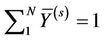 . Operator splitting technique is used to decompose the physical problems, described by Equation (1), into three subprocesses, i.e. the computation of inviscid flux, viscous flux and heat flux. The Equation (1) can be decomposed into two equations as follows
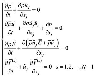 and
and  (2)
(2)
2.2. Algorithm
For the inviscid flux part, the 3D problem can be simplified to the three 1D problems by using dimension splitting technique. For the 1D problem, we applied two-step Lagrange/Remap algorithm to solve equations, and a time step calculation can be divided into four steps: 1) the piecewise parabolic interpolation of physical equations; 2) solving Riemann problems approximately; 3) marching of Lagrange equations; and 4) Remapping the physical quantities to stationary Euler meshes. The more information can be obtained in the author’s literature (Ref. [8,17]). For the viscous flux and heat flux parts, they are calculated by utilizing second-order spatial center difference, two-step Rung-Kutta time marching.
2.3. SGS Stress Models
2.3.1. Smagorinsky SGS Model [12]
The most widely used SGS model is the Smagorinsky model,
 (3)
(3)
where the dimensionless coefficient ,
,  is the model constant, D is the grid-filter width, and
 is the magnitude of the resolved strain rate tensor
 (4)
(4)
2.3.2. Vreman SGS Model [11]
The Vreman SGS model is:
 (5)
(5)
with ,
,![]()
![]() ,
, . The model constant
  is related to the Smagorinsky constant
  by
by  (
( in this paper). The symbol a represents the (3 ´ 3) matrix of derivatives of the filtered velocity
 . If aijaij equals zero,
  is consistently defined as zero. In fact, IIb is an invariant of the matrix b, while aijaij is an invariant of aTa. If the filter width is the same in each direction, then Di=D and b = D2aTa. Like the Smagorinsky model, [18] this model is easy to compute in actual LES, since it does not need more than the local filter width and the first-order derivatives of the velocity field.
2.4. Statistical Properties
A rigorous study of the statistical properties of compressible Richtmyer-Meshkov instability-induced turbulent mixing would need an average several numerical simulations. In practice, it is not possible yet because we are limited by the excessive memory requirements and long run times. So, hereafter, we use only the fine resolution simulation described. Nevertheless, mixing is assumed homogeneous along the transversal y and z direction. Averaged quantities  are then performed along the directions
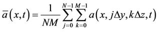 (6)
(6)
For incompressible flows, turbulent fluctuations  of the quantity a are expressed as
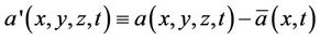 (7)
(7)
On the other hand, for compressible flows, turbulent fluctuations  of the quantity a are expressed within the Favre averaging framework
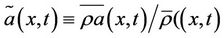 (8)
(8)
3. The SGS Dissipation and Molecular Viscosity Dissipation
In LES the effect of small scales on large scale motions is represented by the SGS stress model. Most of the commonly used SGS models assume that the main function of subgrid scales is to remove energy from the large scales and dissipate it through the action of the viscous forces [19]. It has been known for some years, however, that, on average, energy is transferred from the large scales to the small ones (forward scatter), but reversed energy flow (backscatter) from the small scales to the large ones may also occur intermittently. The most commonly used SGS model, such as the Smagorinsky model, is absolutely dissipative, i.e., it can only account for forward scatter. The other SGS model used in this paper, the Vreman SGS model, is also absolutely dissipative, but it is constructed in such a way that its dissipation is relatively small.
The SGS dissipation, which is the work of SGS stress, represents the energy transport between resolved and subgrid scales, and is defined as [19,20]
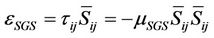 (9)
(9)
If it is negative, the subgrid scales remove energy from the resolved ones (forward scatter); if it is positive, they release energy to the resolved scales (backscatter). It is easy to see that the eddy viscosity SGS models of the Smagorinsky and Vreman type are absolutely dissipative, because the eddy viscosity  is always positive, and yet they are successful in predicting the production and dissipation of SGS energy. The total physical dissipation consists of the molecular viscous, the SGS and the numerical dissipations, but the numerical dissipation will not be discussed here. The absolute value of molecular viscous dissipation is defined as [20]
 (10)
(10)
Figure 1 shows the instantaneous distribution of spanwise-averaged SGS dissipation and molecular viscous dissipation for different SGS models in x direction [21]. This is a RM instability experiment of the evolution of a rectangular block of SF6, and conducted in AWE’s shuck tube [13]. As shown in Figures 1(a) and (b), the molecular viscous dissipation is two magnitudes smaller than the SGS dissipation, so the dissipation is not enough when only the molecular viscosity is considered in the simulation of turbulence. The SGS dissipation of Smagorinsky model is over 1.5 times greater than Vreman model. The dissipation is too great if the Smagorinsky SGS model is used. The SGS dissipation decreases with the turbulence developing. With the simulations, the SGS dissipation and molecular viscosity dissipation have been studied and analyzed. We can see that they have a similar distribution to the large eddy structures. The SGS dissipation is much greater than the molecular viscosity dissipation; the SGS dissipation of Vreman model is smaller than the Smagorinsky model.
4. Comparison of Experiments and Simulations
Peggi’s shock tube experiment model is shown in Figure 2. The tube has a square cross section (80 × 80 mm2). The distance between the initial interface position and the upper end wall is set to 0.3 m. The two gases, the heavy one (SF6) and the light one (air), are initially separated by a plastic membrane. The membrane is broken into small pieces by the passing incident shock wave through the grid. Therefore, the initial wavelengths of the perturbations at the SF6/Air interface are supposed to be of the order of the mesh size. In numerical simulations of MVFT3D, the initial perturbation of the interface is multimode and composed of eight wavelengths l of the order of the experimental wire mesh size: l = 0.5, 0.625, 0.8, 1, 1.25, 1.6, 2, and 2.5 mm, so we take three kinds of random wavelength range of 1.0 mm £ l £ 2.0 mm, 0.5 mm £ l £ 2.5 mm, and 0.1 mm £ l £ 2.9 mm, the average wavelength of álñ =1.5 mm. As we known, before the re-shock, the evolution of the mixing zone width depends
 (a)
(a)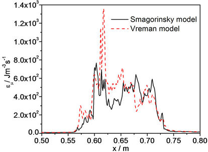 (b)
(b)
Figure 1. Instantaneous distribution of spanwise-averaged SGS dissipation and molecular viscous dissipation for different SGS models in x direction (left column: t = 2846 μs, right column: t = 4046 μs). (a) SGS dissipation; (b) Molecular viscous dissipation.
on the characteristics of the initial perturbations at the interface. So, in our computations, we assume that the wavelengths are of the order of the experimental wire mesh size but we have no experimental information on the amplitude values. So, we arbitrarily take the same value for all the amplitudes of 0.35 mm. The initial shock Mach number is equal to 1.453. The computational model of the

Figure 2. Schematic shock tube and (x, t) diagram.
MVFT3D is shown in Figure 3 and the air, SF6 gas properties are listed in Table 1. The entire fine mesh is done of 800 ´ 200 ´ 200 zones and 32 CPUs are used for parallel computation.
To estimate the mixing zone width from the numerical simulations, we calculate the transversal averaged volume fraction  in each abscissa x, and define the abscissa x between of the
  0.01 and 0.99 as the mixing zone width. Firstly, the experimental model is simulated by using MVFT3D with the Smagorinsky and Vreman SGS models respectively, and with same random wavelength range of 0.5 mm £ l £ 2.5 mm. Figure 4(a) shows the mixing zone width simulated with two SGS models. Dots correspond to the experimental width measured from schlieren pictures in Ref [8]. The error bars of this visual measurement are equal to ±10%. In Figure 4(a), we can see that the difference of mixing zone
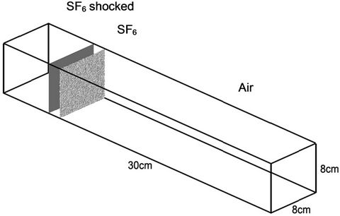
Figure 3. Computational model of the shock tube.
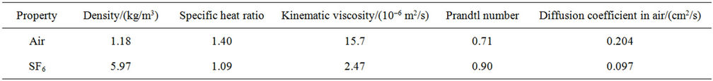
Table 1. Air and SF6 gas properties.
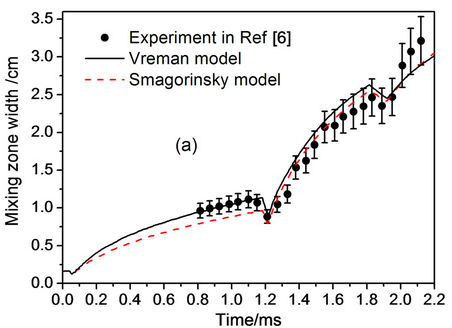
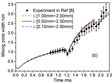
Figure 4. The mixing zone width simulated with two SGS models and three kinds of random wavelength range.
width is from the different SGS models, and the Vreman SGS model is more close to the experiment in whole process. It shows that the Vreman SGS model is superior to the Smagorinsky’s model, and the next simulations are use of it. Secondly, with three kinds of random wavelength range of 1.0 mm £ l £ 2.0 mm, 0.5 mm £ l £ 2.5 mm, 0.1 mm £ l £ 2.9 mm, and Vreman SGS model, the numerical evolution mixing zone width are given in Figure 4(b). It is clear that the difference of mixing zone width from the three kinds of random wavelength range is little, and it’s within the error bars of this visual measurement.
For the Poggi’s experiment simulations, we use the Vreman SGS model and a kind of random wavelength range of 0.5 mm £ l £ 2.5 mm in our MVFT3D. Figure 5 displays the evolution versus time of the experimental and numerical mixing zone widths. In Figure 5, the full line corresponds to mixing zone width value calculated from numerical simulation of MVFT3D. Figure 5 allows us to compare numerical results with experimental ones. After the incident shock passage and before the re-shock, mixing zone widths obtained from numerical simulation is slightly less than experimental ones. And after the first interaction and before the second one, experimental and numerical widths are very similar. Only after the second interaction, the difference is obvious (the experimental almost above 10%). After the incident shock passage and before the first re-shock, the fit of the numerical results gives mixing zone width  for the simulation obtained from MVFT3D, as shown the dash line in Figure 5. Figure 6 displays the turbulent kinetic energy profiles
  at various times. We clearly see the strong generation of turbulent kinetic energy at the incident shock passage through the interface and at the re-shock. Figure 7 gives a zoom of the profiles before the re-shock. The maximum amplitude of these profiles
  decreases by diffusion and dissipation as the mixing zone moves in the shock tube, and it follows
  power law over time and
  power law over space. These results are consistent with Mohamed and Larue approach, that the exponent in the decay power-law for the kinetic energy is equal to 1.3 [22]. After the re-shock, the kinetic energy profiles are larger, see Figure 8, and it is no more easily to find a power-law behavior. Figure 9 gives the volume fraction contour images near the interface at time 0.0 ms, 1.2 ms, 1.8 ms, and 2.2 ms by MVFT3D. From the development and evolution of the disturbed interface, we can see the large-scale
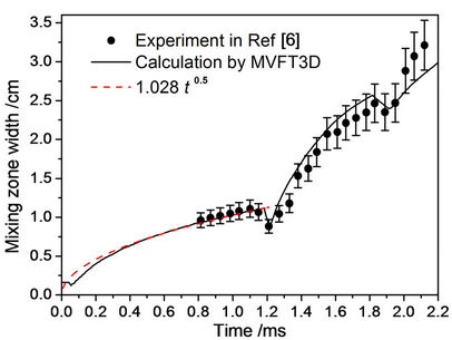
Figure 5. Evolution of the mixing zone width vs. time.
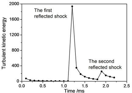
Figure 6. Turbulent kinetic energy vs. time.
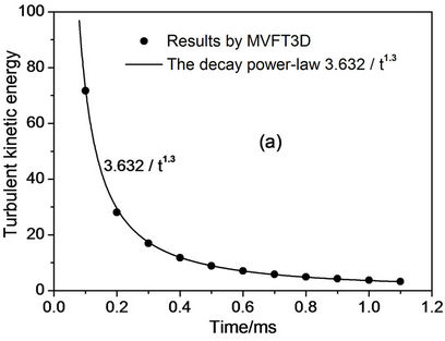
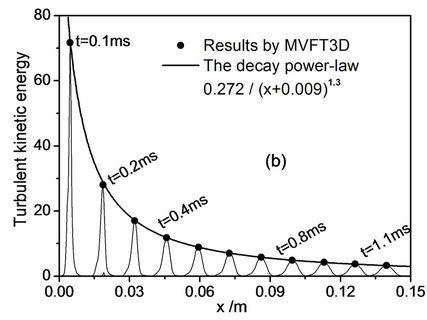
Figure 7. Turbulent kinetic-energy at various times after the incident shock-interface interaction and before the first reflected shock passage.

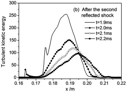
Figure 8. Turbulent kinetic-energy profiles at various times after the first and second reflected shock passage.
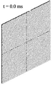
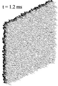
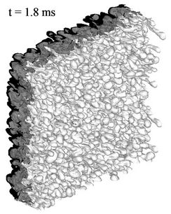
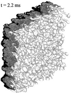
Figure 9. Volume fraction contour images at time 0.0 ms, 0.5 ms, 1.2 ms, 1.5 ms, 1.8 ms, 2.0 ms and 2.2 ms by MVFT3D.
structure of bubbles and spikes have appeared over time, and the bubbles and spikes grow larger continuously. The phenomena of bubble competition appeared, i.e. largescale bubbles merge the small ones around the large ones, and their scales become great larger. This case becomes the main constituents of the mixing zone.
Recently, we simulate the inverse Chevron model from AWE [14] with our MVFT3D. The inverse Chevron was a Richtmyer-Meshkov experiment investigation the mixing at both interface of a dense gas region bounded on either side by air. The computational area is  ,
,  ,
,  . The meshes are 800 ´ 200 ´ 200 and 32 CPUs are used for parallel computation. Gas parameters and random initial perturbation are same with the reference [14]. Here we only give both interfaces of the dense gas volume fraction simulation results of the inverse Chevron model in Figure 10. However, because there is no definite experimental data, we have no quantitative comparison. For the further detailed comparisons will be carried out later in our work.
5. Conclusions
In this paper, an accurate and efficient numerical method and code MVFT3D have been developed for the large eddy simulation of compressible multi-viscous flow and turbulence. An operator splitting technique is used to decompose the physical problems into three sub-processes, i.e. the computation of inviscid flux, viscous flux and heat flux. The Smagorinsky and Vreman subgrid eddy viscosity model are employed to solve the Navier-Stokes equations.
The SGS dissipation and molecular viscosity dissipation have been analyzed in this paper. If molecular dynamic viscosity is only considered in LES of turbulence, the dissipation is not enough while, if the Smagorinsky SGS model is used, the dissipation is too great. In general, when the Vreman SGS model is used in LES, the simulated results are perfect compared with the other two, and the Vreman SGS model is superior to the Smagorinsky’s model in our simulations.
Another main conclusion is the simulations in agreement with Poggi’s experiment for Richtmyer-Meshkov mixing. We have presented the high resolution 3D numerical simulated results of shock-tube experiments of SF6 incident on air performed by Poggi. We can see in numerical simulations the decay of the turbulence before the first reflected shock wave-turbulent mixing zone
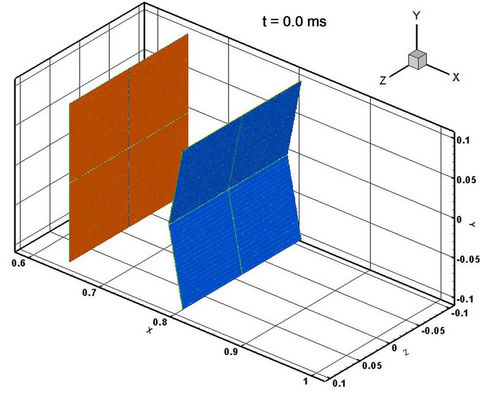

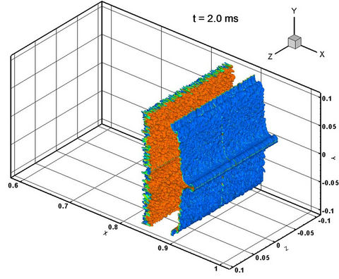
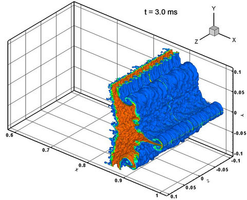
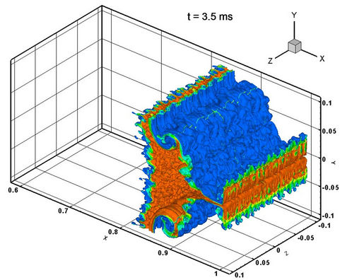
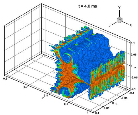
Figure 10. Both interfaces of the dense gas volume fraction simulated results by MVFT3D.
interaction and its strong enhancement by re-shocks. The numerical simulations presented in this paper allow us to characterize and better understand the flow in the Richtmyer-Meshkov instability induced mixing zone.
Finally, the inverse Chevron model from AWE is simulated by MVFT3D.
6. Acknowledgements
The research was sponsored by the National Science Foundation of China Grant No. 11072228 and 11002129, the Science Foundation of China Academy of Engineering Physics Grant No. 2011B0202005 and 2011A0201002, and thanks for the Open Foundation of State Key Laboratory of Advanced Technology for Materials Synthesis and Processing, Wuhan University of Technology.
REFERENCES
- P. B. Putanik, J. G. Oakley, M. H. Anderson and R. Bonazza, “Experimental Study of the Richtmyer-Meshkov Instability Induced by a Mach 3 Shock Wave,” Shock Waves, Vol. 13, No. 6, 2004, pp. 413-429.
- D. Arnett, “The Role of Mixing in Astrophysics,” Astrophysical Journal Supplement Series, Vol. 127, No. 2, 2000, pp. 213-217. doi:10.1086/313364
- M. Boulet and J. Griffond, “Three-Dimensional Numerical Simulation of Experiments on Richtmyer-Meshkov Induced Mixing with Reshock,” 10th International Workshop on the Physics of Compressible Turbulent Mixing (IWPCTM), Paris, 17-21 July 2006.
- V. I. Kozlov, “Simulation of SW/Turbulence Interactions,” 10th International Workshop on the Physics of Compressible Turbulent Mixing (IWPCTM), Paris, 17-21 July 2006.
- B. Thornber, D. Drikakis and D. Youngs, “High Resolution Method for Planar Richtmyer-Meshkov Instabilities,” 10th International Workshop on the Physics of Compressible Turbulent Mixing (IWPCTM), Paris, 17-21 July 2006.
- F. Poggi, M. H. Thorembey and G. Rodriguez, “Velocity Measurements in Turbulent Gaseous Mixtures Induced by Richtmyer-Meshkov Instability,” Physics of Fluids, Vol. 10, No. 11, 1998, pp. 2698-2712. doi:10.1063/1.869794
- M. Claude and G. Serge, “Two-Dimensional NavierStokes Simulations of Gaseous Mixtures Induced by Richtmyer-Meshkov Instability,” Physics of Fluids, Vol. 12, No. 7, 2000, pp. 1783-1798.
- J. S. Bai, J. H. Liu, T. Wang, L. Y. Zou, P. Li and D. W. Tan, “Investigation of the Richtmyer-Meshkov Instability with Double Perturbation Interface in Nonuniform Flows,” Physical Review E, Vol. 81, No. 5, 2010, Article ID: 056302. doi:10.1103/PhysRevE.81.056302
- J. S. Bai, L. Y. Zou, T. Wang, K. Liu, W. B. Huang, J. H. Liu, P. Li, D. W. Tan and C. L. Liu, “Experimental and Numerical Study of the Shcok-Accelerated Elliptic Heavy Gas Cylinders,” Physical Review E, Vol. 82, No. 5, 2010, Article ID: 056318. doi:10.1103/PhysRevE.82.056318
- J. S. Bai, P. Li, T. Wang, B. Xie, M. Zhong and S. H. Chen, “Computation of Compressible Multi-ViscosityFluid Flows,” Explosion and Shock Waves, Vol. 27, No. 6, 2007, pp. 515-521 (in Chinese)
- W. Vreman, “An Eddy-Viscosity Subbgrid-Scale Model for Tubulent Shear Flow: Algebraic Theory and Applications,” Phys fluids, Vol. 16, No. 10, 2004, pp. 3670-3681. doi:10.1063/1.1785131
- J. Smagorinsky, “General Circulation Experiments with the Primitive Equations,” Monthly Weather Review, Vol. 91, No. 3, 1963, pp. 99-164. doi:10.1175/1520-0493(1963)091<0099:GCEWTP>2.3.CO;2
- K. R. Bates, N. Nikiforakis and H. D. Richtmyer-Meshkov, “Instability Induced by the Interaction of a Shock Wave with a Rectangular Block of SF6,” Phys Fluids, Vol. 19, No. 3, 2007, Article ID: 036101, pp. 1-16.
- D. A. Holder and C. J. Barton, “Shock Tube RichtmyerMeshkov Experiments: Inverse Chevron and Half Height,” 9th International Workshop on the Physics of Compressible Turbulent Mixing (IWPCTM), July 2004, p. 43.
- B. Vreman, B. Geurts and H. Kuerten, “Large-Eddy Simulation of the Turbulent Mixing Layer,” Journal of Fluid Mechanics, Vol. 339, 1997, pp. 357-362. doi:10.1017/S0022112097005429
- F. F. Grinstein and G. Karniadakis, “Alternative LES and Hybrid RANS/LES,” Journal of Fluids Engineering, Vol. 124, No. 4, 2002, pp. 821-827. doi:10.1115/1.1518700
- J. S. Bai, T. Wang, L. Y. Zou, et al., “Numerical Simulation of the Hydrodynamic Instability Experiments and Flow Mixing,” Science in China Series G, Vol. 52, No. 12, 2009, pp. 2027-2040. doi:10.1007/s11433-009-0277-9
- D. K. Lilly, “The Representation of Small-Scale Tubulence in Numerical Simulation Experiments,” In: H. H. Goldstine, Ed., Proceedings of IBM Scientific Computing Symposium on Environmental Sciences, Yorktown Heights, New York, 1967, pp. 195-210
- U. Piomelli, W. H. Cabot, P. Moin, et al., “Subgrid-Scale Backscatter in Turbulent and Transitional Flows,” Physical Fluids A, Vol. 3, No. 7, 1991, pp. 1766-1771. doi:10.1063/1.857956
- B. Wang, H. Q. Zhang and X. L. Wang, “On Sub-Grid Scale Turbulence Characteristics,” Engineering Mechanics, Vol. 23, No. 2, 2006, pp. 47-51 (in Chinese).
- T. Wang, J. S. Bai, P. Li and K. Liu, “Large-Eddy Simulations of the Richtmyer-Meshkov Instability of Rectangular Interfaces Accelerated by Shock Waves,” Science China Physics, Mechanics & Astronomy, Vol. 53, No. 5, 2009, pp. 905-914.
- M. S. Mohamed and J. C. Larue, “The Decay Power Law in Grid-Generated Turbulence,” Journal of Fluid Mechanics, Vol. 219, 1990, pp. 195-201. doi:10.1017/S0022112090002919
NOTES
*Corresponding author.