Journal of Transportation Technologies
Vol.3 No.1(2013), Article ID:27024,8 pages DOI:10.4236/jtts.2013.31005
An Induced Demand Model for High Speed 1 in UK
1Department of Civil, Architectural and Environmental Engineering, University of Naples Federico II, Naples, Italy
2School of Civil Engineering and the Environment, University of Southampton, Southampton, UK
Email: fpagliar@unina.it, J.M.Preston@soton.ac.uk
Received November 15, 2012; revised December 16, 2012; accepted December 25, 2012
Keywords: High Speed Rail; Induced Demand; Regression Models; Elasticities
ABSTRACT
Induced travel is an important component of travel demand and increasing attention has been paid to building analytical model to get more precise travel demand forecasting. In general, induced demand can be defined in terms of additional trips that would be made if travel conditions improved (less congested, lower vehicle costs or tolls). In this paper the induced demand resulting from higher design speeds and, therefore by less travel time, for the High Speed 1 in UK will be modelled on the basis of the relationship between existing High Speed Rail demand (dependent variable) to existing High Speed Rail travel times and costs. The covariates include socioeconomic variables related to population and employment in the zones connected by the High Speed Rail services. This model has been calibrated by mean of a before and after study carried on the corridor, when the new High Speed Rail services was introduced. Elasticities of induced travel (trips and VMT) have been computed with respect to fares, travel time and service frequency.
1. Introduction
Investments in High Speed Rail (HSR) systems are currently being undertaken in many countries around the world. These systems represent a closer to optimal solution to meet challenges of increasing mobility demand while simultaneously addressing the greater attention of citizens to sustainability issues. Europe, together with Asia, is already the leader in HSR systems; in fact the development of HSR has been one of the central features of recent European Union transport infrastructure policy. In fact, the programme for the trans-European transport network (TEN-T), introduced under the Treaty of Maastricht, was designed to guarantee optimum mobility and coherence between the various modes of transport in the Union, establishing the key links needed to facilitate transport, optimize the capacity of existing infrastructure, produce specifications for network interoperability, and integrate the environmental dimension [1]. The TEN-T focuses very closely on the development of HSR transport: of the 30 priority projects put forward under this programme, among them 14 concern HSR lines.
In the literature several contributions have been proposed on the empirical analysis of the change of users’travel behaviour after the introduction of HSR services. Most of them have focussed on modelling the mode choice. However very few, as far as the authors know, concentrate on induced demand by HSR [2].
It is well reported in the literature that induced demand is an important component of travel demand, and increasing attention has been paid to building analytical models to get more precise travel demand forecasting. In general, induced demand can be defined in terms of additional trips that would be made if travel conditions improved (less congested, lower vehicle costs or tolls). In this paper the induced demand resulting from higher design speeds and, therefore by less travel time, for High Speed 1 (HS1) in UK will be modelled.
This contribution is organised as follows. In Section 2 an overview on induced demand is presented reporting some case studies present in the literature. Section 3 deals with the case study of HS1 in UK, while Section 4 reports some implications for further research.
2. Induced Demand: An Overview
Modelling induced travel demand is not an easy task due to the high number of variables playing which make the analysis complicated and difficult to generalize. A transportation system is a set of elements interconnected by complex relationships, such as supply sub-system, demand sub-system, residences and activities sub-system; whenever an action is planned on a part of a transportation system, there are unavoidable impacts on other parts, positive or negative. Improvement within the supply sub-system, such as the introduction of a new road infrastructure, of faster/cheaper services, more comfortable vehicles, or in any case actions that increase the utility and/or the satisfaction of the customer about the possibility of moving, create a new share in travel demand [3,4]. Any intervention on a given transport link, producing a mode shift, determines a number of trips which can be split in two parts:
• A diverted demand, that is the number of trips previously carried out by other transport modes, by other route with the same transport mode, or by other services in the same route;
• An induced demand, that is a number of shifts previously not existed and generated directly by the intervention performed [5].
It is difficult to estimate induced traffic with the conventional four-step models, because generation-distribution sub-models are not able to cleave diverted and induced shares; they are also generally not sensitive to changes in the level of service, therefore not able to capture the related effects.
Litman’s contribution [5] provides a comprehensive literature review on the importance of evaluating induced demand brought by road transport. Cervero [6] used data on freeway capacity expansion, traffic volumes, demographic and geographic factors from California between 1980 and 1994. He estimated the long-term elasticity of vehicles-mile-travelled (VMT) with respect to traffic speed to be 0.64, meaning that a 10% increase in speed results in a 6.4% increase in VMT, and that about a quarter of these results from changes in land use (e.g., additional urban fringe development). He estimated that about 80% of additional roadway capacity is filled with additional peak-period travel, about half of which (39%) can be considered the direct result of the added capacity. Duranton and Turner [7] investigated the relationship between interstate highway lane kilometres and highway vehicle-kilometres travelled (VKT) in US cities. They found that VKT increases proportionately to highways and identify three important sources for this extra vehicle travel: increased driving by current residents, an inflow of new residents, and more transport intensive production activity. Time-series travel data for various roadway types indicated an elasticity of vehicle travel with respect to lane miles of 0.5 in the short run, and 0.8 in the long run [8]. This means that half of increased roadway capacity was filled with added travel within about 5 years, and that 80% of the increased roadway capacity will be filled eventually. Noland and Quddus [9] found that increases in road space or traffic signal control systems that smooth traffic flow induced additional vehicle traffic which quickly diminished any initial emission reduction benefits. Small [10] concluded that 50% - 80% of increased highway capacity was soon filled with generated traffic, based on a detailed review of previous studies.
A comprehensive study of the impacts of urban design factors on US vehicle travel found that a 10% increase in urban road density (lane-miles per square mile) increased per capita annual VMT by 0.7% [11]. In a study of eight new urban highways in Texas over several years. Schiffer et al. [12] performed a meta-analysis of induced travel studies to identify shortand long-term elasticities of VMT with respect to changes in traffic lane-miles and other variables. They predicted the amount of VMT induced by regional highway expansion in the Wasatch Front (Salt Lake City region). They concluded that induced travel effects generally decreased with the size of the unit of study.
It is evident how in all the studies stated above, induced traffic has had a strong impact on the expectations of the projects. Most of the benefits estimated, specially about interventions of capacity increase, have been strongly restricted due to filling by induced traffic. It is important within the decision-making process to take into account an induced demand estimation model, for which due to the high number of factors playing (such as kind of roadway, land use, regional or urban area, short or long run effect), the proper adaptation is necessary. Yao and Morikawa [13] developed a model of induced demand resulting from the introduction of a HSR service linking Tokyo, Nagoya and Osaka metropolitan areas in Japan. They proposed an integrated intercity travel demand model with nested structure, including trip generation, destination choice, mode choice and route choice models. Induced demand was estimated introducing an accessibility measure, as an expected maximum utility able to capture the short run behavioural effects such as changes in travel departure times, routes switches, modes switches, longer trips, changes of destination, and new trip generation. They calculated elasticities of induced travel (trips and VMT) with respect to fares, travel time, access time and service frequency for business and non-business travel.
Ben-Akiva et al. [2] modelled the induced demand by HSR in Italy on the basis of the relationship between existing HSR demand (dependent variable) to existing HSR travel times and costs. The covariates include socioeconomic variables related to population and employment in the zones connected by the HSR services. The model was calibrated by mean of a before and after study carried out in the Naples-Rome corridor, where the new HSR services was introduced.
3. The Case Study
High Speed 1 (HS1) is a 108 km (67 mile) HS railway line running from London through Kent to the British end of the Channel Tunnel. Section 1, opened on 28 September 2003, is a 74 km section of HS track from the Channel Tunnel to Fawkham Junction in north Kent. The section’s completion cut the London-Paris journey time by around 21 minutes, to 2 h 35minutes. Section 2 opened on 14 November 2007 and is a 39.4 km stretch of track from the newly built Ebbsfleet station in Kent to London St Pancras. Completion of the section cut journey times by a further 20 minutes (London-Paris in 2 h 15 minutes; London-Brussels in 1 h 51 m) (see Figure 1).
HS 1 railways hosts international services to continental Europe and domestic services to Kent area. Eurostar is the service connecting London with Paris and Brussels across the Channel Tunnel and is provided by Eurostar International Limited, a company owned jointly by London and Continental Railways (40%), the French national railway company Société Nationale des Chemins de fer français (55%), and the Belgian railway operator Nationale Maatschappij der Belgische Spoorwegen (5%). Eurostar services, started in November 2007, have St. Pancras International station as terminal in London, and other calling point in UK are Ebbesfleet International and Ashford International.
Domestic HS services (see Figure 2) are provided by Southeastern Railway Limited, the train operating company holder of the “Integrated Kent Franchise” (1st April 2006 – 31st March 2014). It operates with three kinds of services, which are High Speed, Mainline, and Metro. HS services, begun on December 2009 and they connect London with the Kent using the High Speed 1 to Ebbsfleet and Ashford from which branch off the routes throughout south east of England. Mainline represents the conventional services connecting London with Dover, Canterbury, Maidstone, Thanet, Tunbridge and East Sussex. There are also metropolitan services serving south east and south of London, split in four lines:
• Dartfort and Gravesend metro line
• Hayes metro line
• Orpington and Sevenoaks via Grove Park Metro lines
• Orpington and Sevenoaks via Bromley South Metro lines The number of stations is 179 of which 173 operating and the passenger journeys in 2010/11 were 162.3 million [14].
The introduction of a HSR line naturally leads to travel time savings and may also provide congestion relief for
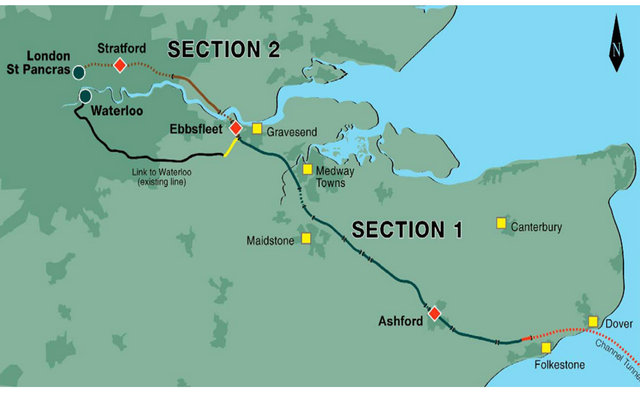
Figure 1. High Speed 1 route map; source: www.lcrhq.co.uk.
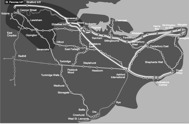
Figure 2. Southeastern route map (grey line is the HS route and the white line represents mainline routes); source: www.southeasternrailway.co.uk.
other transport users on the same corridor. These are, together with the capital and operating costs deriving by the new service, the main impacts on the transport system that several studies have monetised within costbenefit analysis [15,16]. Travel time saving for international trip between London and Paris-Brussels due to the introducing of the HS track is 35 minutes for domestic services between London and Kent using the HS track.
The total time saving benefits, estimated in 2009 by London & Continental Railways (LCR) using the value of time in accordance with WebTAG (the Department for Transport’s website for guidance on the conduct of transport studies) and expressed as a Present Value over 60 years, is 2500 and 1200 for international and domestic respectively.
Concerning congestion relief, LCR assumed a valuation of 40 pence per trip for passengers who switched to the new HS domestic services, and 20 pence for remaining passengers, with an annual growth rate of 1% applied to those values. This approach indicates that, over 60 years as a Present Value, the congestion relief benefit would be £113.6 million. The total construction cost of the line was £5.2 billion (Section 1: £1.9 billion; Section 2: £3.3 billion) and the annual operating cost of around £75 million [16]. The HS fares are on average 30% higher than the conventional, and it was estimated an additional revenue as a Present Value over 60 years of £3.53 billion [10]. The actual use of it is very low, being the service actually running up to 16 trains per day. It is evident that HS1 led to only modest improvements in services between London and Paris/Brussels. The National Audit Office [17] indicated that on transport grounds alone, the case for the HS1 is quite weak, with a Benefit Cost Ratio (BCR) of only 1.1. If regeneration benefits are included (estimated at the time as around £500 million), the BCR is estimated to increase to 1.35, still below the UK Government’s current Value for Money threshold of 1.5. However, recent estimates of regeneration benefits have been as high as £8 billion [18]. Preston and Wall [16] concluded that wider socio-economic impacts are crucial in the justification of HS1 and HSR services more generally.
Data and Methodology
Gravity models are used in social sciences to predict and describe behaviours that mimic gravitational interaction as described in Isaac Newton’s law of gravity [19]. A general application of these models to transport systems analysis concerns demand forecasts in a corridor, expressed as a function of a mass of the origin, a mass of the destination, and a cost function of the shift. Once calibrated applying to all origin/destination (O/D) pairs, these models are able to reproduce generated traffic on a certain corridor in which there has been a change in one or more variable values. Obviously they are not able to cleave diverted and induced demand, because they only take into account what happens on the relations considered. They forecast travel demand changes only on the O/D pairs where a change of the conditions occurred. Therefore the right application of this kind of model depends on the expected transport intervention effects. If diverted traffic, is expected, a generation-distribution model is preferred; when generation effects are expected, a gravity model applied to all O/D pairs is more appropriate. Introducing a new HSR system produces both diverted (from conventional services) and induced traffic; the objective here is to investigate to which results a gravity model leads applied to forecast changes in the number of trips before and after Britain’s HS domestic services introduction. A gravity model to be calibrated needs real travel demand data for conventional and HS services referred to a proper catchment area. Being quite difficult to collect historical travel demand data, the station usage information have been collected, provided by the Office of Rail Regulation (ORR), the independent safety and economic regulator for Britain’s railways. Station usage data represent the total number of trips occurred yearly for each Britain’s railway station. Being the vast majority of the travels concerning HS services towards London metropolitan area, it has been considered a catchment area made up by a number of origins equal to the number of stations served by HS services, and London as the only destination. Socioeconomic variables have been at first considered, but the low sample size and the unavailability of a precise catchment area led to very low statistical significant results.
The first step has been the analysis of the HSR services running from London to Kent, provided by the Southeastern Train Operating Company. These services involve 24 stations throughout Kent area, each of which is served by both HS and conventional trains.
Referring to the current timetable available on the Southeastern website, the following information have been computed for each station:
• The number of HS trains per day to London;
• The mean HS journey time to London;
• The mean HS fare to London;
• The number of conventional trains per day to London;
• The mean conventional journey time to London;
• The mean conventional fare to London.
The mean fare is the average of the full fares ranging in the day and the same values are deducted from the travelcard discount (34%).
The second step has been that of finding a correlation between the station usage provided by ORR, and a set of variables linked by the following function:
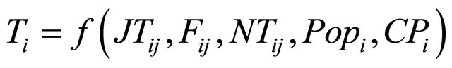 (1)
(1)
where:
i, j is the considered station and London respectively;
Ti is the number of trips in station i;
JTij is the journey travel time between i, j;
Fij is the fare between i, j;
NTij is the number of trains between i, j;
Popi is the population within 4 minutes uncongested driving time from station i;
CPi is the number of car parking spaces available in station i.
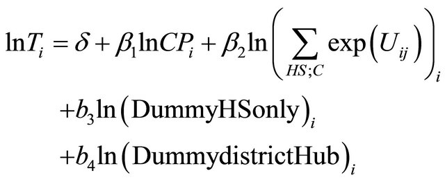 (2)
(2)
where:
d is the intercept;
Ti is the number of trips in station i;
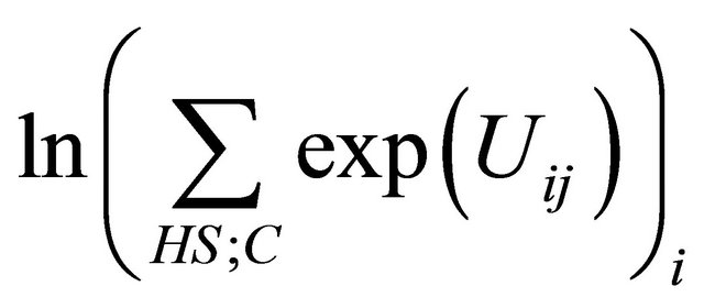 is the Logsum (3)
The Logsum is a measure of the user’s satisfaction with respect to the available alternatives. It has been computed (for each station toward London) as a generalized journey time (see Equation 4), then used together with the fare for obtaining a utility value (see Equation 6) both for HS and conventional services.
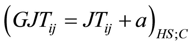 (4)
(4)
where:
GJTij is the generalized journey time;
JTij is the in vehicle time (mean journey time)
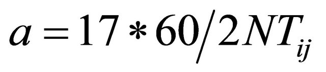 (5)
(5)
a is the average waiting time in minutes considering 17 hours of service per day;
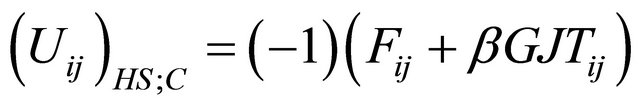 (6)
(6)
b = 11.7247 pounds/hour (value of time derived by Webtag).
(DummyHSonly)i is a dummy variable which assumes the value 1 for the stations served by HS services only, and the value 0 for the stations served by both HS and conventional services.
(DummydistrictHub)i is a dummy variable which assumes the value 1 for the expected main District station, in terms of number of customer services, opportunity to make interchange, centrality in respect to the District area; the value 0 for the other stations. The regression outputs are shown Table 1.
The coefficients of the regression estimated are all statistically significant and to test the model accuracy a comparison has been made between the predictions of the model and the real values. Given the station usage data for the years 2008/09, 2009/10, and 2010/11, it has been calculated the real percentage change of the number of trips before the domestic HS (2008/09-2009/10) and after its introduction (2009/10-2010/11). It should be pointed out that 2009/10 data are considered before the HS introduction because they are referred to the financial year, and so they include only three months of HS services (started in December 2009). Forecast of the number of trips for 2008/09 is calculated considering in the model the Logsum related to 2008 timetable from where the mean journey time and the number of trains to London for each station have been calculated. The fares have been estimated starting by the current values considering the Retail Price Index and the annual fares increase. The value of time annual change (see Table 2) has been obtained from WebTAG.
Concerning the 2009/10 model prediction, the Logsum is calculated with the approximation of considering the current conventional timetable in place of 2009/10 values. As it can be seen in the Table 3, the real change in the number of trips from 2008/09 to 2009/10 is generally negative, except for Rochester and Canterbury West.
Table 1. Regression results.
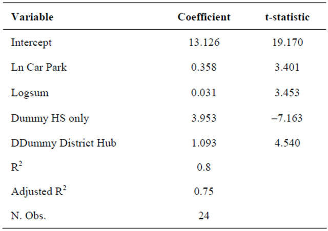
Table 2. Value of time adopted.
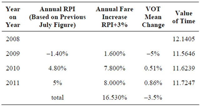
Table 3. Comparison between model forecast and real data before High Speed 1.
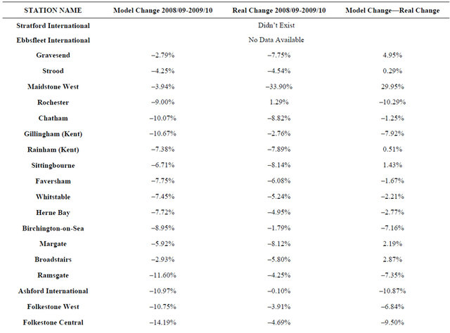
Recession is certainly one of the reasons, but the prediction of the model reflects well the negative trend even if it does not take into account crisis effects. That is because the Logsum decreases from 2008/09 to 2009/10, first because of the fare increases, second because of the number of stops increase that has led to higher travel times.
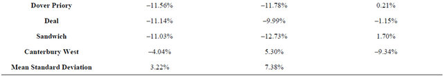
As it can be seen the lower accuracy is for Maidstone West with a 30% error, and for Canterbury Westand Rochester, where the model predicts respectively a decrease of 4% and 9% against an increase of 5.3% and 1.3%, and for Ashford and Folkestone Central, with 10.87% and 9.5% error respectively. Besides the approximation concerning the 2009/10 Logsum, that likely would have led to more precise results, there are other factors which could have been taken into account. Firstly, the more or less influence of the crisis on the areas, difficult to take into account without reliable local GDP data; secondly, it could be a substantially different value of time from that adopted; thirdly, socioeconomic variable as the population, employees etc have not been considered. A further comparison has been made between the change in number of real trips and those predicted from 2009/10 to 2010/11 (see Table 4). This could also represent an approximate measure of the extent to which HSR has grown the market.
Even in this case there are values in which the forecast is substantially different from the real data, such as Strood, Rochester, Folkestone West and Canterbury West, and the reasons are similar to those stated above.
Table 4. Comparison between model forecast and real data before and after high speed 1.
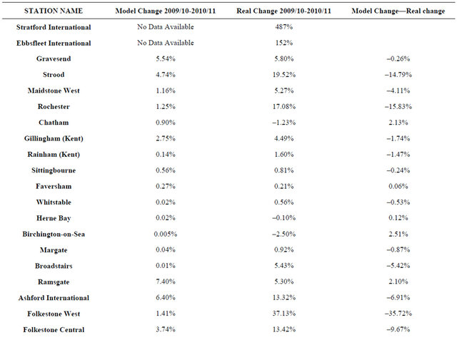
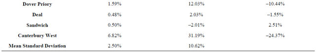
Ebbsfleet and Stratford stations are charecterized by high real changes because 2009/10 data include only three months of HS service, which is the only service available for them. The model is therefore not able to predict the number of trips for 2009/10 because there is not the Logsum measure related to the conventional service. This is a consequence of the approximation of considering the station as origin, instead of the classic area’s centroids.
As the model is linear with respect to the Logsum variable, the elasticity related to the latter has been computed as:
 (7)
(7)
It follows that increasing the Logsum of one unit, the number of trips will increase of 3.15%. A more immediate measure is the elasticity with respect to the fare and the generalized journey time, from where the Logsum is derived. Obviously there are two elasticity values, for both conventional HS services.
Concerning the generalized journey time, which is the sum of in-vehicle time and average waiting time, the elasticity is –0.06 for conventional trains and –0.14 for HS trains; this means that a 10% increase in journey time results in a 0.6% decrease in conventional number of trips, and a 1.4% decrease in a HS number of trips. Elasticity with respect to the fare is –0.05 for conventional and 0.34 for HS; meaning that a 10% increase in journey time results in a 0.5% decrease in the number of trips for conventional and a 3.4% decrease for the HS number of trips.
4. Conclusions and Further Perspectives
Modelling induced demand by HSR systems is a topic not well-established in the literature, this paper attempts to provide a contribution to the international research. The model specified has been used to predict the change in the number of trips between two years and with the purpose of comparing the results with the real available data. There are two possible implications for this model:
• It could be used to forecast the change in the number of trips deriving by the change in time and fare on a corridor where two services, HS and conventional are available;
• It could be used to predict the number of trips deriving by the introduction of a new HS service.
In any case, an improvement in the level of services variables is reflected in a customer satisfaction increase (modelled by the Logsum variable), and the related elasticity indicates that a 1 unit increase results in a 3.15% increase in the number of trips.
The main constraint of this study is related to the unavailability of a conventional catchment area, to which always transport analysis is referred, besides the unavailability of the real travel demand data. These limitations also can be found in the exclusion in the regression models of some socio-economic variables such as population and employment, as well as other transport variables such as car journey times and costs. Further perspectives will consider the inclusion of such variables in the models.
REFERENCES
- European Union, “High-Speed Europe, a Sustainable Link between Citizens,” 2010. http://ec.europa.eu/research/horizon2020/index_en.cfm
- M. Ben-Akiva, E. Cascetta, P. Coppola, A. Papola and V. Velardi, “High Speed Rail Demand Forecasting: Italian Case Study,” Proceedings of the WCTR Conference, Lisbon, 11-15 July 2010, 9 p.
- M. Ben-Akiva and S. Lerman, “Discrete Choice Analysis,” The MIT Press, Cambridge, 1985.
- E. Cascetta, “Transportation Systems Analysis: Models and Applications,” Springer, New York, 2009. doi:10.1007/978-0-387-75857-2
- T. Litman, “Generated Traffic and Induced Travel, Implications for Transport Planning—Report for the Victoria Transport Institute,” 2011. http://www.vtpi.org/gentraf.pdf
- R. Cervero, “Road Expansion, Urban Growth, and Induced Travel: A Path Analysis,” Journal of the American Planning Association, Vol. 69, No. 2, 2003, pp. 145-163. doi:10.1080/01944360308976303
- G. Duranton and M. A. Turner, “The Fundamental Law of Road Congestion: Evidence from US Cities,” Working Paper 370, University of Toronto, Toronto, 2008.
- R. B. Noland, “Relationships between Highway Capacity and Induced Vehicle Travel,” Transportation Research Part A: Policy and Practice, Vol. 35, No. 1, 2001, pp. 47- 72. doi:10.1016/S0965-8564(99)00047-6
- R. Noland and M. A. Quddus, “Flow Improvements and Vehicle Emissions: Effects of Trip Generation and Emission Control Technology,” Transportation Research Part D: Transport and Environment, Vol. 11, No. 1, 2006, pp. 1-14. doi:10.1016/j.trd.2005.06.003
- K. A. Small, “Urban Transportation Economics,” Harwood (Chur), Anne Arundel, 1992.
- L. C. Barr, “Testing for the Significance of Induced Highway Travel Demand in Metropolitan Areas,” Transportation Research Record, Vol. 1706, 2000, pp. 1-8. doi:10.3141/1706-01
- R. G. Schiffer, M. W. Steinvorth and R. T. Milam, “Comparative Evaluations on the Elasticity of Travel Demand, Committee on Transportation Demand Forecasting,” 2005. www.trbforecasting.org/papers/2005/ADB40/05-0313_Schiffer.pdf
- E. Yao and T. Morikawa, “A Study on Integrated Intercity Travel Demand Model,” Transportation Research Part A: Policy and Practice, Vol. 39, No. 4, 2005, pp. 367-381. doi:10.1016/j.tra.2004.12.003
- Office of Rail Regulation, “National Rail Trends 2010/11 Yearbook,” 2011. http://www.rail-reg.gov.uk/
- LCR (London & Continental Railways), “Economic Impact of High Speed 1, Report,” 2009. http://www.lcrhq.co.uk/
- J. M. Preston and G. Wall, “The Ex-Ante and Ex-Post Economic and Social Impacts of the Introduction of HighSpeed Trains in the South-East of England,” Planning Practice and Research, Vol. 23, No. 3, 2008, pp. 403-422. doi:10.1080/02697450802423641
- National Audit Office, “The Channel Tunnel Rail Link. HC 302,” The Stationery Office, London, 2008. http://www.nao.org.uk/
- Dft, Transport Analysis Guidance, “UK Department for Transport,” 2007. http://www.dft.gov.uk/
- A. G. Wilson, “Entropy in Urban and Regional Modelling: Retrospect and Prospect,” Geographical Analysis, Vol. 42, No. 4, 2010, pp. 364-394.