Open Journal of Optimization
Vol.2 No.3(2013), Article ID:36842,6 pages DOI:10.4236/ojop.2013.23012
On the Quadratic Transportation Problem
1University of Baltimore, Baltimore, MD, USA
2Department of Transportation, Middletown, CT, USA
Email: vadlakha@ubalt.edu, Krys.Kowalski@po.state.ct.us
Copyright © 2013 Veena Adlakha, Krzysztof Kowalski. This is an open access article distributed under the Creative Commons Attribution License, which permits unrestricted use, distribution, and reproduction in any medium, provided the original work is properly cited.
Received May 23, 2013; revised June 30, 2013; accepted July 19, 2013
Keywords: Quadratic Cost Function; Transportation Problem; Direct Method; Dynamic Shadow Prices
ABSTRACT
We present a direct analytical algorithm for solving transportation problems with quadratic function cost coefficients. The algorithm uses the concept of absolute points developed by the authors in earlier works. The versatility of the proposed algorithm is evidenced by the fact that quadratic functions are often used as approximations for other functions, as in, for example, regression analysis. As compared with the earlier international methods for quadratic transportation problem (QTP) which are based on the Lagrangian relaxation approach, the proposed algorithm helps to understand the structure of the QTP better and can guide in managerial decisions. We present a numerical example to illustrate the application of the proposed method.
1. Introduction
The classical transportation problem (TP) is a wellstructured problem that has been studied extensively in the literature. The TP deals with the distribution of goods from m suppliers (sources) to n customers (destinations). Each of the m suppliers can ship to any of the n customers at a shipping cost per unit cij (unit cost for shipping from supplier i to customer j). Each supplier has ai units of supply and each customer has a demand of bj units. The objective is to schedule shipments from sources to destinations so that total transportation cost, ∑∑cijxij, is minimized. A typical TP is formulated as follows:
Minimize
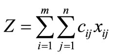 (1)
(1)
subject to
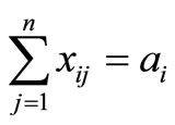 for i = 1, 2, …, m (2)
 for j = 1, 2, …, n (3)
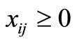 for all (i, j).
Like the TP, the quadratic transportation problem (QTP) can be stated as a distribution problem where each of the m suppliers can ship units to any of the n customers at cost fij(xij) and where fij(xij) is a quadratic function of xij, the amount shipped from source i to destination j. The objective is to minimize the total transportation cost while meeting demand at the destinations.
Mathematically, a QTP is formulated as:
Problem QTP:
Minimize
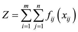 (4)
(4)
subject to
 for i = 1, 2, …, m, (5)
 for j = 1, 2, …, n, (6)
 (7)
(7)
 ;
;  (8)
(8)
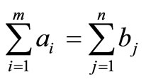
 , integer One constraint out of Equations (5) and (6) is redundant if the QTP is balanced, i.e., if Equation (7) is satisfied. Note that, as with a classical TP, we assume nonnegative conditions and zero value of cost functions at 0. As compared with the linear TP, the QTP provides a superior representation of real live distribution problem where the unit cost of transportation is not constant. For example, consider the case where the unit cost of transportation might decrease with the volume of transported goods. Conversely, there may be an opposite situation where the unit cost of transportation increases with volume due to highway congestion.
There is no efficient direct algorithm to solve Problem QTP available in the literature. Some authors have attempted to solve Problem QTP as a quadratic program with a quadratic objective function involving (m * n) variables subjected to (m + n) linear conditions. The problem thus formulated could then be solved using the theory of Lagrange multipliers. Such a process, however, is very cumbersome, as it requires taking partial derivatives with respect to each of the (m * n) variables and (m + n − 1) Lagrange multipliers, and solving the resulting (m * n) + (m + n − 1) equations. This task could be overwhelming even for a small QTP. And with a second-degree polynomial function, one cannot even be sure whether the point obtained is a local minimum or the global minimum. Many current software programs for solving QTP are based on various algorithm developed in the literature based on Lagrange multipliers. Authors experimented with some of these: Lindo, Excel, and WinQSB. In several instances, the three programs provided different results, affirming the inability of these algorithms to always provide the global minimum for a QTP.
Quadratic functions are versatile, as they can be used as approximations for many other functions, as with regression analyses and have been used to model special scheduling problems. In this paper we propose a novel direct analytical method to solve a QTP where the cost coefficients are quadratic functions. The proposed algorithm exploits the properties of absolute points developed by Adlakha and Kowalski [1] to solve a TP with linear costs. It is easy to apply and provide insight into the problem, and with this, we are able to critically analyze the problem. The algorithm can also be used as a preprocessor to reduce the transportation problem size.
2. Literature Review
Research on TP has generally addressed situations where linear costs are assumed. In such a case, a TP can be formulated as a linear program and solved by the regular simplex (big-M), the dual simplex method or even an interior approach. However, these algorithms require additional variables, which complicate the formulation, enlarge the tableaux, and increase the number of iterations. These problems led to the stepping-stone (SS) technique, which—as a network-oriented algorithm— proved very successful and became the standard technique for over 60 years. In practice, however, the SS algorithm encounters major obstacles, including difficulties in identifying an initial basic feasible solution, resolving SS degeneracy, and enumerating SS paths [2]. Literature is filled with efforts to overcome these deficiencies and improve the SS algorithm [3-8]. Korukoğlu and Balli [9] propose a variant of Vogel’s Approximation Method (VAM) to obtain efficient initial solutions for large scale transportation problems. Other researchers [1, 10] provide alternative solution algorithms.
Variations in TP cost functions have been studied by many researchers. Szwarc [11] develops a method for solving TPs with cost coefficients of the form cij = ui + vj, where ui and vj represent nonnegative real numbers, a method that has applications in shop loading and aggregate scheduling. Along the same lines, with applications to stock location and information storage, Evans [12] considers TPs in which cost coefficients are factorable, that is, cij = uivj. Evans demonstrates that if the rows are arranged by non-increasing ui, and the columns by nondecreasing vj, then the northwest corner rule provides an optimal solution.
A limited number of researchers have worked on quadratic programming problems. Hochbaum et al. [13] consider a specialized scheduling problem. They formulate the problem as an integer program with a quadratic, non-separable objective and transportation constraints. Employing methods of real analysis, they prove a tight proximity result between the integer solution to that problem and a fractional solution of a related polynomially solvable problem. Megiddo and Tamir [14] consider separable quadratic problems including separable convex QTP with a fixed number of sources. Using the technique of Lagrangian relaxation, they provide linear algorithms based on the multidimensional procedures developed by the authors. Cosares and Hochbaum [15] present a linear algorithm for the continuous QTP with two source nodes.
To mention a few other related works, Eduardo et al. [16] develop a productivity index for the case of a cost model using a quadratic cost function. Wanner et al. [17] propose a local search optimizer as an additional operator in multi-objective evolutionary techniques, to help find more precise estimates of the Pareto-optimal surface with a smaller cost-of-function evaluation. The operator employs quadratic approximations of the objective functions and constraints for the purpose of enhancing local search phase. Lu et al. [18] present a long-step infeasible primal-dual path-following algorithm for convex quadratic programming (CQP) whose search directions are computed by means of a preconditioned iterative linear solver.
3. The Quadratic Transportation Problem
Before we proceed, we reiterate some terminology from the TP literature. A location (i, j) is said to be loaded (or occupied) if there is a value assigned to it in the solution. Location (i, j) is said to be fully loaded if that value equals min(ai, bj), i.e., the assignment exhausts supply ai at source i and/or demand bj at destination j. Location (i, j) is interchangeably referred to as cell (i, j).
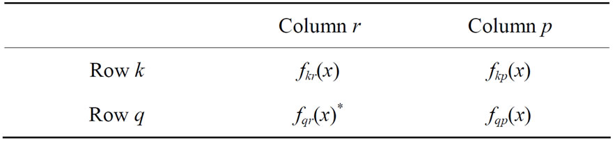
Stepping-stone (SS) chains are commonly used in solution procedures for TPs. An SS chain at a cell, (q, r), of a TP cost matrix refers to an ordered sequence of at least four cells such that 1) any two consecutive cells lie in either the same row or the same column, 2) no three consecutive cells lie in the same row or column, and 3) the last cell in the sequence has a row or column in common with cell (q, r). Tables 1(a) and (b) provide examples of SS chains involving 4 and 6 cells, respectively, where xij denotes the load at cell (i, j). Note that the allocation of any load at cell (q, r) affects the loads at all cells in the SS chain at cell (q, r).
3.1. Absolute Points for the QTP
Definition 1: An absolute point (AP) is a cell (q, r) in a QTP that must be occupied in any optimal solution within the interval from 0 to the smaller of the values aq and br.
The procedure for finding an AP is based on the following assumptions:
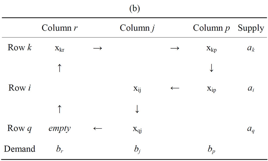
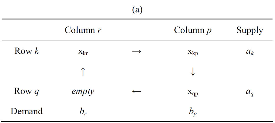
Table 1. (a) An Example of an SS Chain of Four Cells; (b) An Example of an SS Chain of Six Cells.
1) There is a cell (q, r) in a QTP that must be occupied in any optimal solution within the interval from 0 to the smaller of the values aq and br, i.e., an AP exists.
2) If such a cell (q, r) were excluded in a given distribution, i.e., not loaded, then there exists an SS chain leading to cell (q, r) from every other cell that is occupied.
Suppose cell (q, r) is an AP. Then this cell (q, r) must be loaded with a shipment from supply aq and demand br to eliminate the cell (q, r) from future computations. Not loading it means that, for every other loading in row q and column r, there will be an SS chain leading to cell (q, r). So we have to prove the existence of an SS chain leading to (q, r) from every other cell in row q and column r. If we ignore cell (q, r), we have to load other cells in row q and column r, for example cells (k, r) and (q, p), to satisfy demand and supply requirements.
If there is an SS chain leading to a cell (q, r), then, to guarantee a gain from this transaction, we must have
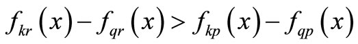
 (9)
(9)
For a given q and r, if inequality (9) holds for every k = 1, 2, …, m, and every p = 1, 2, …, n, then (q, r) is an AP location, and the value {fkr(x) – fqr(x)} is the largest of the comparisons between rows k and q. Note that the left-hand side of (9) represents the penalty for placing assignments at locations (k, r) and (q, p) rather than at location (q, r). See Adlakha and Kowalski [1] for details on identifying an absolute point for a classical TP. What follows are the steps for identifying an AP in a QTP with cost functions fij(x). These steps involve pivoting on the qth row in the first QTP cost matrix.
Step AP1: Calculate fijq(x) = fqj(x) – fij(x), i = 1, 2, … m, j = 1, 2, … n. Ignore the qth row as otherwise we would be comparing it with itself.
Step AP2: Draw all n quadratic curves fijq(x) on the same graph, i = 1, 2 … m, i ¹ q.
Step AP3:
Step AP4: An AP exists if the minimum functions in each row are in the same column.
Remark 1: For Step AP2, many software packages are easily available to draw the quadratic curves and to study the ranges.
Remark 2: For Step AP3, to determine the minimum element fiq(x), one should simply limit the search to the range of 0 to min(aq, bj) for j = 1, 2, … n. There is no need to exceed the range min(aq, bj) as this is the maximum load that can be assigned at cell (q, j).
3.2. Absolute Quadratic Algorithm for the QTP
The algorithm identifies the AP cells, which are loaded sequentially, and the QTP is reduced. It is obvious from the absolute point theory that if a cell were an AP, loading it would have no impact on the distribution of the remaining loads. Note that once an AP is identified, it is clear from inequality (9) that the AP has to be loaded with the maximum possible amount.
Step 1: Look for AP cells along each row.
Step 2: If none, go to Step 6. Otherwise continue.
Step 3: For each AP cell (q, r), assign xqr = min(aq, br). Change aq ® (aq - xqr), br ® (br - xqr).
Step 4: If modified ai or bj = 0, delete the corresponding ith row or jth column.
Step 5: If the above analysis yields a solution, STOP. Otherwise go back to Step 1 with the reduced cost matrix.
Step 6: Find a solution to the reduced cost matrix using any inductive method.
4. A Numerical Example
We illustrate the Absolute Point Algorithm for the QTP with the example presented in Table 2.
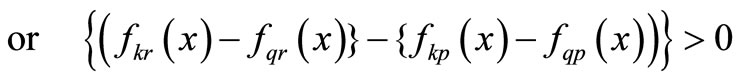
Step 1: First we search for available APs in the cost matrix. Step AP1 provides the following three fijq(x) = fqj(x) – fij(x) matrices by pivoting on rows i = 1, 2, and 3. Figure 1 presents fijq(x) functions and curves corresponding to Step AP2 directly under each fijq(x) matrix for each i. Since there are only three rows, each fijq(x) matrix has only two sets of differences fqj(x) – fij(x). The graphs related to pivoting on row 1 are provided directly beneath the fij1(x) matrix where graph fij1,i(x) presents the set of three quadratic equations in the ith row of fij1(x),
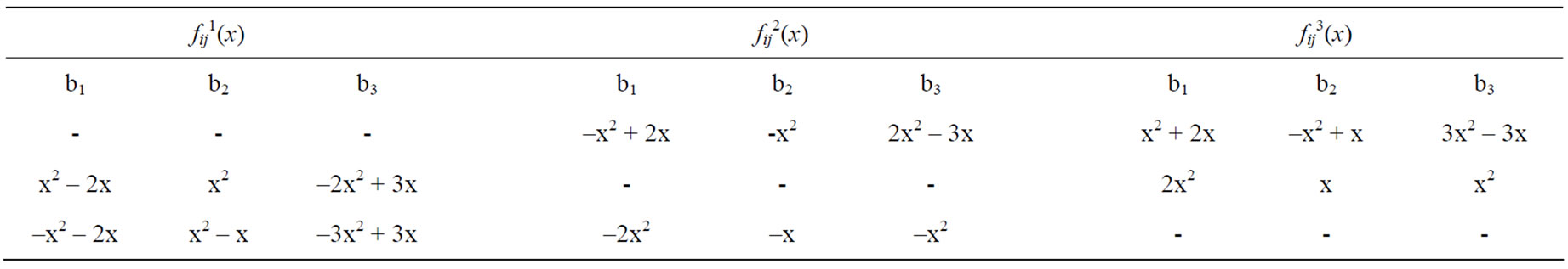
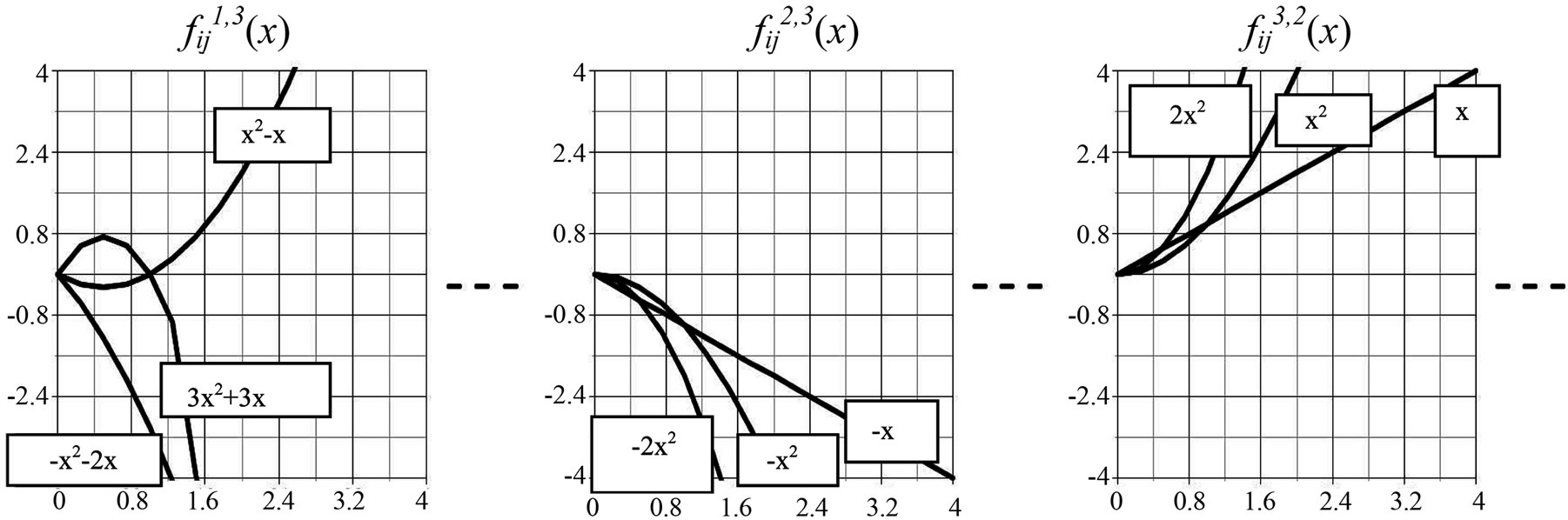
Figure 1. Step AP2: fijq(x) functions and curves for the example.
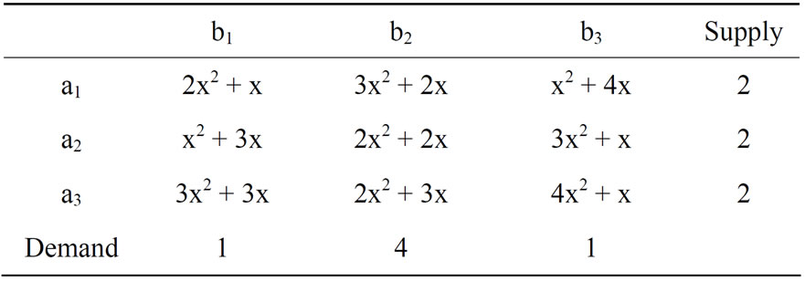
Table 2. Cost matrix fij(x) for the QTP example.
and so on.
1) Step AP3: Looking at the two curves under fij1(x), we find that the smallest function in fij1,2(x) is f211(x) = x2-2x for 0 £ x £ 1; and the smallest function in fij,1,3(x) is f311(x) = –x2 – 2x for 0£ x £1 where min(a1, b1) = 1. Step AP4: Since minimum functions f211(x) and f311(x) are in the first column, Step AP5 indicates that cell (1, 1) is an AP.
2) Similarly looking at the two curves under fij3(x), we find that the smallest function in fij3,1(x) is f133(x) =3x2 – 3x for 0 £ x £ 1; and the smallest function in fij3,2(x) is f233(x) = x2 for 0£ x £1 where min(a3, b3) = 1. Since minimum functions f133(x) and f233(x) are in the third column, cell (3, 3) is an AP.
Step 3:
1) For AP cell (1, 1), assign x11 = min(a1, b1) = 1. Change a1 ® (a1 − 1) = 1; b1 ® (b1 − 1) = 0.
2) For AP cell (3, 3), assign x33 = min(a3, b3) = 1. Change a3 ® (a3 − 1) = 1; b3 ® (b3 − 1) = 0.
Step 4: Since modified b1 = 0 and b3 = 0, delete the corresponding first and third columns.
Step 6: The remaining supplies are easily assigned to the only remaining column—the second column—to meet the demand b2 = 4 units. Table 3 presents the resulting solution with a total cost of 30 for shipping 6 units.
Note that the conditions for APs for the analyzed formulation are dynamic and depend both on the values of the function cost coefficients and on the demand and supply values. This means, for example, that a given AP location can stop being an AP for a different set of the demand and supply values.
Shadow Prices for the QTP
Arsham [2] discusses the relationship between the shadow prices and the optimal solution of a TP. Using a similar analogy, we utilize the shadow price theory to verify the optimality of a QTP solution. The shadow functions and prices are easily obtained from a QTP solution matrix as follows:
1) Set ui + vj = fij(xij) for all loaded cells.
2) Set v1 (or another ui or vj) = 0 and solve the system of equations for all ui and vj values.
3) Compute the shadow function for each unused cell (i, j) as ui + vj.
According to established TP shadow price theory, the current QTP solution is optimal if all ui + vj function values obtained in step (iii) above are all less than or equal to the corresponding fij(xij) values. Table 4 presents the shadow functions for the solution obtained in Table 3 where the loaded cells are marked by *. It is clear that for all currently unused cells the value of the shadow function/price is less than or equal to the corresponding quadratic cost functions from Table 2 if any value greater than 0 and less than the maximum possible value, min(ai, bj), is assigned at the cell. This confirms that the solution obtained in Table 3 is optimal.
5. Conclusions
We have developed a direct solution algorithm for solving a QTP. The Absolute Quadratic Algorithm is based on various intrinsic characteristics of the QTP. It looks for cells and routes that will always be used in an optimal solution because of cost efficiency, regardless of supply and demand constraints. Since an absolute point must always be loaded in any optimal solution, loading it exhausts either a supply or demand. Upon depleting the corresponding row or column, the proposed method also reduces the dimensions of the cost matrix for the QTP. After reductions and eliminations, the solution of the QTP is “squeezed” into the remaining cells and may be determined logically in the last step. We extend the shadow price theory of the TP to the QTP and develop a shadow function matrix to verify optimality.
To the best of our knowledge, besides the very laborious Lagrangian method, this algorithm is the first for providing a direct solution of a QTP. As compared with the earlier international methods for QTP which are based on the Lagrangian relaxation approach, the proposed algo

Table 3. Optimal solution for 3 × 3 QTP.
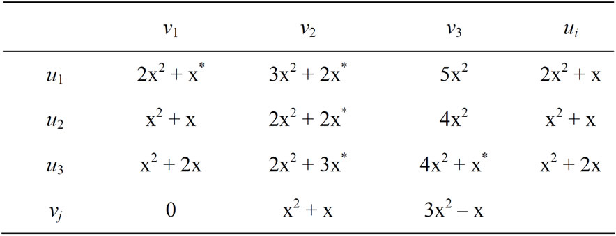
Table 4. Shadow Price Matrix for the QTP Example.
rithm helps to understand the structure of the QTP better and can guide in managerial decisions. Future work should seek to extend the theory to coefficients represented by higher degree polynomials. Because such functions can have local minima, a gradient-type algorithm can fail to obtain the global minimum. It is, of course, possible that a QTP may not have any APs. In such a case, other methods or estimations, including heuristics, can be used, and the shadow price analysis can be used to confirm optimality. Future research is needed to develop other generally applicable methods.
REFERENCES
- V. Adlakha and K. Kowalski, “An Alternative Solution Algorithm for Certain Transportation Problems,” International Journal of Mathematical Education in Science and Technology, Vol. 30, No. 5, 1999, pp. 719-728. doi:10.1080/002073999287716
- H. Arsham, “Postoptimality Analysis of the Transportation Problem,” JORS: Journal of the Operational Research Society, Vol. 43, No. 2, 1992, pp. 121-139.
- S. K. Goyal, “Improving VAM for Unbalanced Problems,” JORS, Journal of the Operational Research Society, Vol. 35, No. 12, 1984, pp. 1113-1114.
- J. Intrator and W. Szwarc, “An Inductive Property of Transportation Problem,” Asia-Pacific Journal of Operational Research Society, Vol. 5, 1988, pp. 79-83.
- M. A. Hakim, “An Alternative Method to Find Initial Basic Feasible Solution of a Transportation Problem,” Annals of Pure and Applied Mathematics, Vol. 1, No. 2, 2012, pp. 203-209.
- A. Shafaat and S. K. Goyal, “Resolution of Degeneracy in Transportation Problems,” Journal of the Operational Research Society, Vol. 39, No. 4, 1988, pp. 411-413.
- A. Sultan, “Heuristic for Finding an Initial B. F. S. in a Transportation Problem,” Opsearch, Vol. 25, 1988, pp. 197-199.
- C. E. Wilsdon, “A Simple, Easily Programmed Method for Locating Rook’s Tours in the Transportation Problem,” Journal of the Operational Research Society, Vol. 41, No. 9, 1990, pp. 879-880.
- S. Korukoğlu and S. Balli, “An Improved Vogel’s Approximation Method for the Transportation Problem,” Mathematical and Computational Applications, Vol. 16, No. 2, 2011, pp. 370-381.
- V. Adlakha and H. Arsham, “Simplifying Teaching the Transportation Problem,” International Journal of Mathematical Education in Science and Technology, Vol. 29, No. 2, 1998, pp. 271-285. doi:10.1080/0020739980290210
- W. Szwarc, “Instant Transportation Solutions,” Naval Research Logistics Quarterly, Vol. 22, No. 3, 1975, pp. 427- 440. doi:10.1002/nav.3800220303
- J. R. Evans, “The Factored Transportation Problem,” Management Science, Vol. 30, No. 8, 1984, pp. 1021- 1025. doi:10.1287/mnsc.30.8.1021
- D. S. Hochbaum, R. Shamir and J. G. Shanthikumar, “A Polynomial Algorithm for an Integer Quadratic NonSeparable Transportation Problem,” Mathematical Programming, Vol. 55, No. 1-3, 1992, pp. 359-371.
- N. Megiddo and A. Tamir, “Linear Time Algorithms for Some Separable Quadratic Programming Problems,” Operations Research Letters, Vol. 13, No. 4, 1993, pp. 203- 211. doi:10.1016/0167-6377(93)90041-E
- S. Cosares and D. S. Hochbaum, “Strongly Polynomial Algorithms for the Quadratic Transportation Problems with a Fixed Number of Sources,” Mathematics of Operations Research, Vol. 19, No. 1, 1994, pp. 94-111. doi:10.1287/moor.19.1.94
- M. B. Eduardo, S. J. D. Francisco and J. R. Real, “Adapting Productivity Theory to the Quadratic Cost Function, An application to the Spanish electric sector,” Journal of Productivity Analysis, Vol. 20, No. 2, 2003, pp. 233-249.
- E. F. Wanner, F. G. Guimaraes, R. H. C. Takahashi and P. J. Fleming, “Local Search with Quadratic Approximations into Memetic Algorithms for Optimization with Multiple Criteria,” Evolutionary Computation, Vol. 16, No. 2, 2008, pp. 185-224. doi:10.1162/evco.2008.16.2.185
- Z. Lu, R. D. C. Monteiro and J. W. O’Neal, “An Iterative Solver-Based Long-Step Infeasible Primal-Dual PathFollowing Algorithm for Convex QP Based on a Class of Preconditioners,” Optimization Methods & Software, Vol. 24, No. 1, 2009, pp. 123-143. doi:10.1080/10556780802414049