International Journal of Modern Nonlinear Theory and Application
Vol.04 No.01(2015), Article ID:54881,39 pages
10.4236/ijmnta.2015.41005
The Boundary Layer Equations and a Dimensional Split Method for Navier-Stokes Equations in Exterior Domain of a Spheroid and Ellipsoid
Jian Su1, Hongzhou Fan2, Weibing Feng3, Hao Chen4, Kaitai Li1
1School of Mathematics and Statistic, Xi’an Jiaotong University, Xi’an, China
2School of Energy and Power Engineering, Xi’an Jiaotong University, Xi’an, China
3School of Computer Engineering and Science, Shanghai University, Shanghai, China
4School of Mechanics and Engineering, Southwest Jiaotong University, Chengdu, China
Email: ktli@mail.xjtu.edu.cn
Copyright © 2015 by authors and Scientific Research Publishing Inc.
This work is licensed under the Creative Commons Attribution International License (CC BY).
http://creativecommons.org/licenses/by/4.0/


Received 22 February 2015; accepted 15 March 2015; published 20 March 2015
ABSTRACT
In this paper, the boundary layer equations (abbreviation BLE) for exterior flow around an obstacle are established using semi-geodesic coordinate system (S-coordinate) based on the curved two dimensional surface of the obstacle. BLE are nonlinear partial differential equations on unknown normal viscous stress tensor and pressure on the obstacle and the existence of solution of BLE is proved. In addition a dimensional split method for dimensional three Navier-Stokes equations is established by applying several 2D-3C partial differential equations on two dimensional manifolds to approach 3D Navier-Stokes equations. The examples for the exterior flow around spheroid and ellipsoid are presents here.
Keywords:
Boundary Layer Equations, Dimensional Split Method, Navier-Stokes Equations, Dimensional Two Manifold

1. Introduction
In computational fluid dynamics, one need to compute the drag exerted on a body in flow field; in particular, optimal shape design has received considerable attention already, see Li and Huang [1] , Li, Chen and Yu [2] , and Li, Su, Huang [3] . It has become vast enough to branch into several disciplines on the theoretical side, many results deal with the existence of solutions to the problem or its relaxed form, on the practical side, topological shape  optimization which solves numerically the relaxed problem or by local shape variation. In this case
we have to compute the velocity gradient  along the normal to the surface of the boundary and normal
stress tensor  to the surface. All those computation have to do in the boundary layer. Therefore this leads to make very fine mash; for example, 80% nodes will be concentred in a neighborhood of the surface of the body.
In this paper a boundary layer equations for  on the surface will be established using local
semi-geodesic coordinate system based on the surface, provide the computational formula for the drag func- tional. In addition, a dimensional split method for three dimensional Navier-Stokes equations is established by applying several 2D-3C partial differential equations on the two dimensional manifolds to approximate 3D Navier-Stokes equation.
The Dimensional Slitting Methods deal, for examples, with thin domain problem as elastic shell (see Ciarlet [4] , Li, Zhang and Huang [5] ), Temam and Ziane [6] , and with boundary value problem with complexity boun- dary geometry (see [7] -[10] ).
The content of the paper is organized as the followings. Section 2 establishes semi-geodesic coordinate system and related the Navier-Stokes equations; Section 3 assumes that the solutions of Navier-Stokes equa- tions in the boundary layer can be made Taylor expansion with respect to transverse variable, derive the equations for the terms of Taylor expansion; Section 4 proves the existence of the solutions of the BLE; Section 5 provides the computational formula of the drag functional; Section 6 provide a dimensional splitting method for 3D Navier-Stokes equations; Section 7 provide some examples.
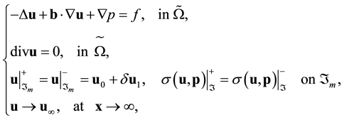
2. Navier-Stokes Equations and Its Variational Formulation in a Semi-Geodesic Coordinate System
Through this paper, we consider state steady incompressible Navier-Stokes equations and its variational formu- lation in a thin domain , a strip with thickness
 ![]() and by a Lipchsitz continuous boundary
and by a Lipchsitz continuous boundary
![]() ,
,
![]() (2.1)
(2.1)
or
![]() (2.1')
(2.1')
which are invariant form in any curvilinear coordinate system. Let
![]()
At first, we introduce semi-geodesic coordinate system (abbreviation S-coordinate). As well known thhat boundary layer ![]() in 3D Euclidean space bounded by
in 3D Euclidean space bounded by ![]() and
and ![]() where
where ![]() is bottom of the boundary layer, a surface of solid boundary of the flow fluid, and
is bottom of the boundary layer, a surface of solid boundary of the flow fluid, and ![]() is a top boundary of
is a top boundary of , an artificial interface of the flow fluid where
  is unit normal vector to
  and
and  is a parameter, the
thickness of the strip, the boundary layer. Assume that there exits a smooth immersion  such that
  are linearly independent where
  is a Lipschitz domain with boundary
  and
and  are parameters which are called Gaussian coordinate on the surface
 . It is
obvious that  are basis. So the geometry of the surface
  is given by first fundamental form and second
fundamental form and third fundamental form which coefficients are metric tensor  and curvature tensor
  and tensor
  respectively where
  is unit normal vector to

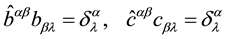
Their contravariant components  are given by

What’s follows that we will frequently used the inverse matrix  of
of :
:
Now, assume that there exists an unique normal vector  to
to  from each point
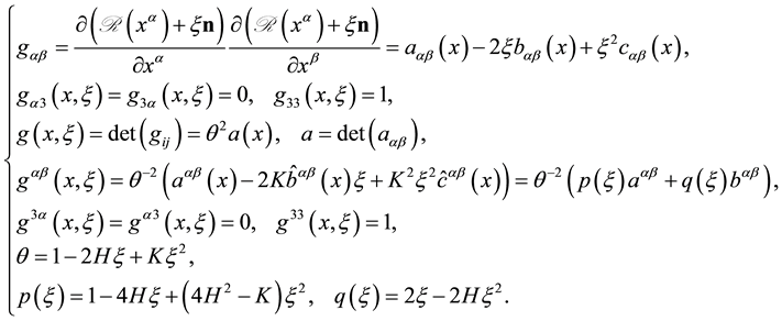
  such that (see Figure 1)

where  is origin. Thereby, point
  is determined by triple numbers
 . Inversely, a triple numbers
  can determine uniquely a point
 . Curvilinear coordinate
  in
in 
is called semi-geodesic coordinate based on the surface . Its bases vectors are
  and the metric tensor
  of 3D Euclidean space
  in this semi-geodesic coordinate are given by

Therefore, the metric tensor of  can be expressed by the metric tensor of
  in the semi-geodesic coor- dinate system:
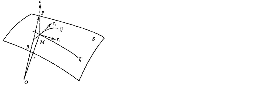
Figure 1. The diagram of semi-geodesic coor- dinate system.
 (2.2)
(2.2)
(see ref. [1] ) wherre  are mean curvature and Gaussian curvature of
 . Throughout this paper, we employ semi-geodesic coordinate system
  based on the surface
  (see [1] and Figure 1) (later
on, denote  -coordinate). The metric tensor of
  in this coordinate are denoted by
 . It is obvious that the determinate
  if
if  is small enough. Hence coordinate
  is nonsingular.
In addition, we review the main notation. Greek indices and exponents belong to the set , while Latin indices and exponents (except when otherwise indicated, as when they are used to index sequences) belong to the set
 , and the summation convention with respect to repeated indices and exponents is systematically
used. Symbols such as  or
or  designate the Kronecker’s symbol. The Euclidean scalar product and the the exterior product of
  are noted
  and
and ; the Euclidean norm of
  is noted
 . Fur-
thermore, the physical or geometric quantities with the asterisk  express the quantities on the manifold
 , for example,
  is covariant derivative on
 . Furthermore, the physical or geometric quantities with the asterisk
  express the quantities on the manifold
 , for example,
  is covariant derivative on
 . Further- more, the notations
  are given contravariant components and covariant components of the permuta- tion tensor on
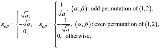
There are following relations of the first,second and third fundamental forms (ref. [1] )

The following give the relations of differential operators in the space and on  (see [1] ). For example, under the
  -coordinate system, the Christoffel symbols of
  and
and  satisfy

and covariant derivatives of the vector field are given by
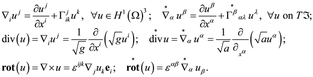
where ![]() is covariant component of vector
is covariant component of vector![]() . The strain tensor of vector field in
. The strain tensor of vector field in ![]() and on
and on ![]() are given by respectively
are given by respectively
![]()
Of course,![]() ;
; ![]() Under the
Under the ![]() -coordinate system there are following formula for the covariant derivatives of the vectors in the space
-coordinate system there are following formula for the covariant derivatives of the vectors in the space ![]() and on the
and on the ![]() (ref. [1] )
(ref. [1] )
![]() (2.3)
(2.3)
The strain tensors of the vectors in ![]() and on
and on ![]() can be expressed as
can be expressed as
![]() (2.4)
(2.4)
where
![]() (2.5)
(2.5)
In the semi-geodesic coordinate system (see next section), define the bilinear form ![]() and trilinear form
and trilinear form ![]()
![]() (2.6)
(2.6)
Then, the primitive variable variational formulation for Navier-Stokes Equations (2.1') is given by
![]() (2.7)
(2.7)
while the Navier-Stokes Equations (2.7) in semi-geodesic coordinate system are expressed as
![]() (2.8)
(2.8)
![]() (2.9)
(2.9)
3. Boundary Layer Equations
Assume that ![]() is a two dimensional manifold parameterized by
is a two dimensional manifold parameterized by![]() . In the neighborhood of the orientate surface
. In the neighborhood of the orientate surface ![]() let define a surface
let define a surface![]() :
:
![]()
It is obvious that ![]() ia a geodesic parallel surface of
ia a geodesic parallel surface of ![]() and the geodesic distance each other is equal to
and the geodesic distance each other is equal to ![]() where
where ![]() is a small constant.In this paper we only consider exterior flow around a body occupied by
is a small constant.In this paper we only consider exterior flow around a body occupied by ![]() with a two dimensional manifold
with a two dimensional manifold ![]() without boundary. The boundary layer domain
without boundary. The boundary layer domain
![]()
Domain ![]() is called the “stream layer”.
is called the “stream layer”.
Assumption AI assume that the solutions ![]() of Navier-Stokes Equation (2.7) in boundary layer
of Navier-Stokes Equation (2.7) in boundary layer ![]() in semi-geodesic coordinate system and right term
in semi-geodesic coordinate system and right term ![]() can be made Taylor expansion with respect to the transverse variable
can be made Taylor expansion with respect to the transverse variable ![]()
![]() (3.1)
(3.1)
In same time, the test vector also can be made Taylor expansion
![]()
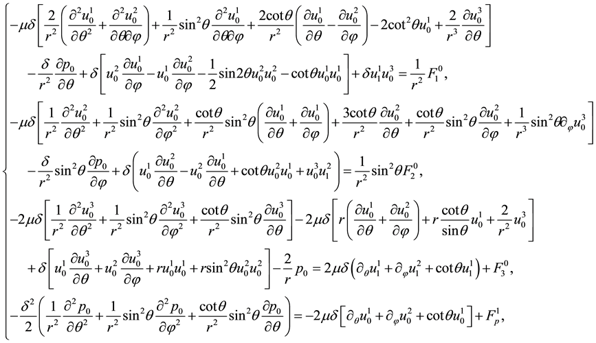
Theorem 1 In a boundary layer domain ![]() with non-slip boundary condition
with non-slip boundary condition![]() , if the Assumption AI (3.1) is satisfied, then nine unknown of
, if the Assumption AI (3.1) is satisfied, then nine unknown of ![]() satisfy following a system of three partial dif- ferential equations which are called boundary layer equations I (BLE I):
satisfy following a system of three partial dif- ferential equations which are called boundary layer equations I (BLE I):
![]() (3.2)
(3.2)
and five algebraic equations
![]() (3.3)
(3.3)
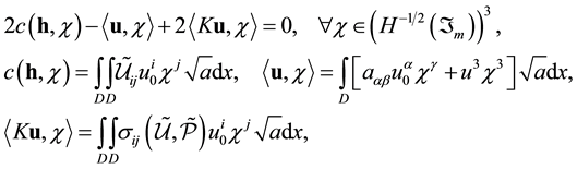
Associated variational formulations with (3.2) is given by
![]() (3.4)
(3.4)
where the bilinear forms defined by
![]() (3.5)
(3.5)
![]()
and
![]() (3.6)
(3.6)
where
![]()
![]() is normal stress tensor at
is normal stress tensor at ![]() (top boundary of boundary layer),
(top boundary of boundary layer), ![]() are defined by (3.1).
are defined by (3.1).
Next, let consider interface equation. In this case ![]() is a flexible surface (slip and passing through conditions).
is a flexible surface (slip and passing through conditions).
Assumption AII Assume that the solutions ![]() of Navier-Stokes Equation (2.1) in stream layer
of Navier-Stokes Equation (2.1) in stream layer
![]() in semi-geodesic coordinate system based on
in semi-geodesic coordinate system based on ![]() and right term
and right term ![]() can be made Taylor expansion with respect to the transverse variable
can be made Taylor expansion with respect to the transverse variable ![]()
![]() (3.7)
(3.7)
Theorem 2 Assume that the Assumption II is satisfied. Then six unknown of ![]() in (3.7) satisfy following system of the nonlinear partial differential equations which are called stream layer equations II (abbreviation SLE II) (interface equations):
in (3.7) satisfy following system of the nonlinear partial differential equations which are called stream layer equations II (abbreviation SLE II) (interface equations):
![]() (3.8)
(3.8)
![]() (3.9)
(3.9)
The right terms
![]() (3.10)
(3.10)
In particular, for flexible (slip condition![]() ) boundary surface
) boundary surface![]() , neglect hight order terms and keep one order term of
, neglect hight order terms and keep one order term of![]() , then (3.3) (3.4) and (3.5) become
, then (3.3) (3.4) and (3.5) become
The Proof of Theorems 1 and 2 is neglected.
4. The Existence of the Solution
In this section we prove the existence of the weak solution of (3.2). To do that we consider variational
formulation of (3.2). Let ![]() where
where ![]() is a sobolev space of 1-order with perio-
is a sobolev space of 1-order with perio-
dic boundary condition. Since ([14] , Th.1.8.6) we claim
![]()
where
![]()
Let define bilinear form:![]() ,
,
![]() (4.1)
(4.1)
where ![]() are two positive constants and
are two positive constants and ![]() and
and
![]()
Then corresponding variational formulation for (3.2) is given by
![]() (4.2)
(4.2)
where
![]() (4.3)
(4.3)
Lemma 1 Assume that the metric tensor and curvature tensor of ![]() satisfy
satisfy ![]() and
and ![]() respectively. Then viscosity tensor of
respectively. Then viscosity tensor of ![]()
![]() and metric tensor
and metric tensor ![]() are positive definition, i.e. for any symmetric matrix
are positive definition, i.e. for any symmetric matrix![]() , there exists two constants
, there exists two constants![]() ,
, ![]() independent of
independent of ![]() such that
such that
![]() (4.4)
(4.4)
Therefore,
![]() (4.5)
(4.5)
Furthermore, If ![]() and the thickness
and the thickness ![]() of boundary domain small enough, then bilinear form
of boundary domain small enough, then bilinear form ![]() is positive
is positive
![]() (4.6)
(4.6)
Proof The proof of (4.4) can be found in ([1] [4] ). It remain to prove (4.6). By virtue of the positive definition of metric tensor ![]() and assumption of lemma and using Hoelder inequality, we assert that
and assumption of lemma and using Hoelder inequality, we assert that
![]()
where ![]() is a constant independent of
is a constant independent of ![]() depending
depending![]() . The proof is complete.
. The proof is complete. ![]()
Lemma 2 Assume that the two-dimensional manifold  is smooth enough such that the metric tensor
  of
of  and curvature tensor
  satisfy
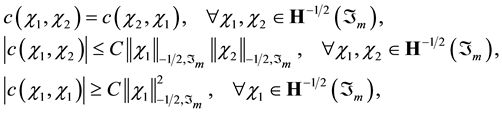
 . Then the bilinear forms
  defined by (4.1):
  is symmetric, continuous
 (4.7)
(4.7)
where  Furthermore if
  is smaller enough such that
 (4.8)
(4.8)
then they are also coercive respectively
 (4.9)
(4.9)
where  is a constant independent of
  having different meaning at different place and

Proof Indeed it is enough to prove the coerciveness (4.8) since the continuous and symmetric are obvious by Hoelder inequality. Since Lemma 1,

In view of Korn inequality on Riemann manifold (see [4] Th.1.7.9 )

we assert that
 (4.10)
if  satisfies
  To sum up, we conclude our proof.
Next we consider variational problem (4.2) corresponding to boundary layer Equation (3.4). Let
 (4.11)
Lemma 3 Assume that the manifold  satisfies that
  such that there exists a constant

The thickness  of the boundary layer is small enough. Then bilinear form
  defined by (4.11) is continuous:
 (4.12)
where  and also satisfies following inequality
 (4.13)
where  is small enough and parameters
  satisfy
 (4.14)
Proof It is easy to verify (4.12) by applying Hoelder inequality and Poincare inequality. It remains to prove (4.13). At the first, we recall that the assumptions of the lemma shows
Taking (4.8) into account, from (4.10) it infers
 (4.15)
(1) Since Lemma 1 and (4.3) we have

Moreover, using Godazzi formula , we obtain

Therefore

Thanks to

 (4.16)
We assert that

Second inequality shows
 (4.17)
Using Young inequality

we have
 (4.18)
By similar manner,
 (4.19)
 (4.20)
Substituting (4.18-4.20) into (4.16) leads to
 (4.21)
Taking (4.9) into account, it yield
 (4.22)
If
 (4.23)
Then
 (4.24)
It is easy to verify that (4.23) is satisfied if the parameters  in the definition (4.1) are held
 (4.25)
Next we consider trilinear form. Taking into account of

we claim that

By Ladyzhenskya inequality (Temam [11] )
 (4.26)
it infers that
 (4.27)
Combing (4.15) (4.24) and (4.27), we obtain
 (4.28)
This complete our proof. 
Theorem 3 Assume that the hypotheses in Lemma 3 are satisfied and the mapping

is sequentially weakly continuous in 

Then there exists at least one solution  of (4.2) satisfying
 (4.29)
where  is the thickness of boundary layer,
  are constants defined in the followings.
Proof We begin with constructing a sequence of approximate solutions by Galerkin’s method. Since the space  is a separable Hilbert space, there exist sequence
  in
in  such that: 1) for all
 , the elements
  are linearly independent; 2) the finite linear combinations of the
  are dense in
 . Such sequence
  are called a basis of the separable space. Denote by
  the subspace of
  spanned by finite sequence
 . Then we solve an approximate problem of (4.2)
 (4.30)
Setting

Problem (4.30) is equivalent to a system of nonlinear equations with m unknowns . For each
  problem (4.30) has at least one solution. In fact, when defining a mapping
  by
by

where  is the scalar product in
 ,
,  is a solution of problem (4.30) if only if
  Since
Since

it follows from (4.28)

Let  Furthermore, assume that
 (4.31)
if  is small enough. Then
 (4.32)
if
 (4.33)
Hence, we conclude
 (4.34)
Moreover,  is continuous in a finite dimension space
 , we can apply following lemma ([12] ).
Lemma 4 Let  be a finite dimensional Hilbert space whose scalar product is denoted by
  and the corresponding norm by
 . Let
. Let  be a continuous mapping from
  into
into  with the following property: there exists
  such that
 (4.35)
Then, there exists an element  in
in  such that
 (4.36)
Therefore there exists a solution  for problem (4.30) with
 (4.37)
This shows that the sequence ( of the solutions to (4.30) in
  are uniformly bounded. Therefore we can extract a subsequence (still denoted by
 ) such that

Then, the compactness of the embedding of  into
into  implies that

Since  is dense in
 , it is obvious that if

Taking the limit of both sides of (4.30) implies

therefore

Then  is a solution of (4.2) and which satisfies

The proof is complete. 
Remark The mapping  is sequentially weakly continuous in
  can be found in [3] .
5. Dimensional Split Method for Exterior Flow Problem around an Obstacle and a Two Scale Parallel Algorithms
In this section, we proposal a dimensional split algorithm for the three dimensional exterior flow around a obstacle occupied by .
.  is a smooth surface of the obstacle and
 . Assume that
  is decomposed by a series of geometric parallel surfaces
  into a series of stream layer
  bounded by
  such that
 .
.
On every surface , it generalis a global system including one system of BLE I on the boundary surface
  of the obstacle and N-1 systems of flexible boundary equations BLE II on
 :
:

where right terms are given by

The features of these systems are that the right terms of them depend upon the solution of next system, for example, the right term of kth-system depend upon the solution of  th. system. It is better to apply alterative iteration algorithm to solve these systems. That is
(1) Suppose that right hands , are known;
(2) Solve system of 
(3) Modifying  by using results obtained , then goto (2) to be continuous until reach certainly accuracy.
In order to find solution of Navier-Stokes equations at any point P in Exterior domain 
(i) Identify point P in which stream layer  bounded by
 , then set
  in local coordinate system;
(ii) 
where  are solution of BLE on
 .
.
In details,
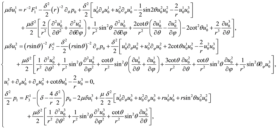
(I) For  i.e. solid surface with non-slip boundary condition, we give the boundary layer equations BLE I (3.2) on the boundary surface
  of obstacle. from Theorem 2, three unknown
  solve
solve
 (5.1)
(5.1)
and six unknown  can be found by six algebraic equations
 (5.2)
(5.2)
Associated variational formulations with (5.1) is given by
 (5.3)
(5.3)
where  are two positive arbitrary constants, the bilinear forms and trilinear form are
 (5.4)
(5.4)
and
 (5.5)
(5.5)
The right terms are given by
 (5.6)
(5.6)
where .
.
(II) For , i.e. on flexible surfaces, corresponding boundary layer equations SLE II (for
 ) at flexible surface (artificial interface)
 ,
,  are given by (3.8) and (3.9)
 (5.7)
(5.7)
 (5.8)
(5.8)
 (5.9)
(5.9)
On the other hand we can improve (5.7). To do that, making covariant derivative  on both sides of the first equation in (3.9) and combining last equation in (3.9),
  can be found by
 (5.10)
 (5.11)
The variational formulations corresponding to (5.7) and (5.1) are given respectively by
 (5.12)
and
 (5.12')
where the bilinear forms and linear form are defined by
 (5.13)
(III) For  i.e. a last artificial interface Surface
 . There are two choices to do that (1) assume that
  on
on  where
where  is known infinity up stream flow velocity. (2) we assume that the flow outside
  is governed by Oseen equation and give a boundary integrating equation on
  via fundamental solution of Oseen equations.
(1) Let  is Cartesian coordinate and
  where
where  are base vectors. The surface
  can be parametrization by
  where
where  are parameters, i.e. are Gaussian
coordinate on . Then base vectors
  and unit normal vector
  in semi-coordinate on
  are given by
 (5.14)
while the metric tensor  and curvature tensor
  are given
 (5.15)
where . Our aim is to give boundary conditions on
 . Owing to (4.12) we claim
On other hand, we show

Indeed,
Finally we imply
 (5.16)
where  is describing
 . (5.16) will be used for solving BLE I on
  with
with .
.
(2). Let assume that the flow outside of  is governed by Oseen equation
 (5.17)
 is known and
  is a well known vector, for example
 , and
, and , and
, and  are solutions of 2D-3C Navier-Stokes equations on the
 . Furthermore,
  is normal stress tensor to be found in the section. Let
  be a Cartesian coordinate.
  are fundamental solutions of the follow- ing equations
 (5.18)
 can be expressed as
 (5.19)
where  is a fundamental solution of following equation
 (5.20)
where for 
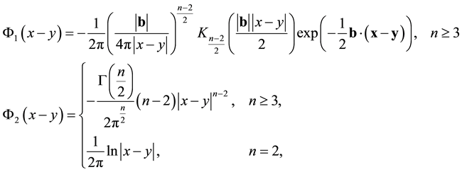 (5.21)
where  is a Bessel function of second kind.
Then integral expressions of solutions of Oseen problem (5.9) are given by
 (5.22)
where  is stress tensor


Here we employ Cartesian coordinate system  and artificial surface
  is a two
dimensional manifold. The integrate representation (5.17) of the solution of Oseen problem is invariant, it is valid for any curvature coordinate. Since formula for fundamental solution  is represent at Cartesian coordinate. It also can be compute at any curvature coordinate according transformation rule of tensor of one order.
Vector  in (5.17) is normal stress tensor at
 The normal stress tensor
  at
at  is continuous
 . This means that
  on both sides of
  are coincidental.
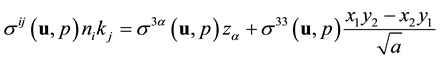
Normal stress tensor  on the artificial boundary
  satisfies following equation
 (5.23)
(5.23) can be rewrite in semi-geodesic coordinate based on :
:
 (5.24)
where,  is semi-geodesic coordinate. By the transformation of coordinate,
  where
where  are Cartesian coordinate and
  is the parametrization representation of the surface
 .
.
Lemma 5 The bilinear form  defined by (5.23) is symmetric, continuous and coercive from
  into
into 
Theorem 4 Assume that  are smooth and bounded in
  Then there exists a unique solution of following variational problem
 (5.25)
Parallel algorithms. The Domain ia made partition by m interfaces surfaces and we obtain  the systems of BLE I and SLE II. Solving each BLE I and SLE II independently, then applying alternatively iterative algorithm are performance at the same time. On the other hand, the parallel algorithms for BLE I and SLE II can be used. Therefore, parallel algorithms are applied in two direction at the same time.
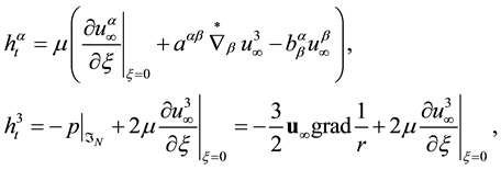
6. Computation of the Drag
The drag is a force exerted on a solid boundary surface, for example, . There is normal stress on
  which can expressed under semi-geodesic coordinate based on
  by
by

The drag is a projection of normal stress on the direction of infinite stream flow . Hence
 (6.1)
(6.1)
Since unit normal vector at  is
is  and by (5.1)
 (6.2)
(6.2)
Therefore
As well known that the stress tensor is given by

At surface 


Since

because of

Hence
 (6.3)
(6.3)
The drag is a force exerted on a solid boundary surface, for example, . There is normal stress on
  which can be expressed under semi-geodesic coordinate based on
  by
by . The drag is a pro- jection of normal stress on the direction of infinite stream flow
 . Hence
 (6.4)
(6.4)
where  are parameter representation of
 .
.
7. Examples
7.1. The Flow around a Sphere
Assume that  and
and  are Cartesian and spherical coordinates respectively

Simple calculations show that the metric tensor of spherical surface . is given
 (7.1)
(7.1)
The tensor of second fundamental form, i.e. curvature tensor of spherical surface is given by
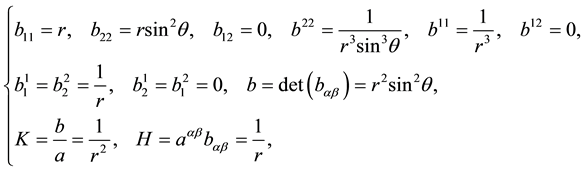 (7.2)
(7.2)
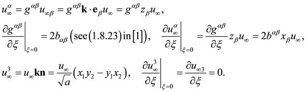
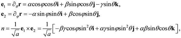
the base vectors of semi-geophysical coordinate system are given
 (7.3)
(7.3)
We remainder have to give the covariant derivatives of the velocity field, Laplace-Betrami operator and trace-Laplace operator. To do this we have to give the first and second kind of Christoffel symbols on the spherical surface  as a two dimensional manifolds

Then covariant derivatives of vector  on the two dimensional manifold
  is given by

Nonlinear terms

and

The associated Laplace-Betrami operator and divergence operator on  are given by
 (7.4)
(7.4)
while trace-Laplace operator on 
 (7.5)
(7.5)
(A) BLE I
Substituting previous formula into Theorem 1 we assert that
 (7.6)
(7.6)
In particular, if the flow is axial symmetric then
 (7.7)
(7.7)
where

(5.7) is a two points boundary value problem for ordinary differential equations.
 (7.8)
(7.8)
 (7.9)
(7.9)
(B) SLE II
The first, we note
So that

Taking (5.7) into account, we claim that
(7.10)
If the flow is symmetric then
 (7.11)
and
(7.12)
where
 (7.13)
The drag is given by
 (7.14)
7.2. The Flow around an Ellipsoid
Let parametric equation of the ellipsoid be given by
 (7.15)
where  are Cartesian basis,
  are the parameters and
  are called Guassian co- ordinates of ellipsoid. The base vectors on the ellipsoid
The metric tensor of the ellipsoid is given by
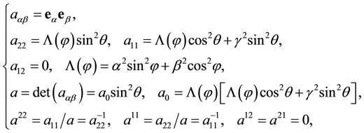 (7.16)
Curvature tensor, mean curvature and Gaussian curvature are given by
 (7.17)
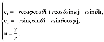
Semi-Geodesic Coordinate System Based on Ellipsoid 
That is

The radial vector at any point in 


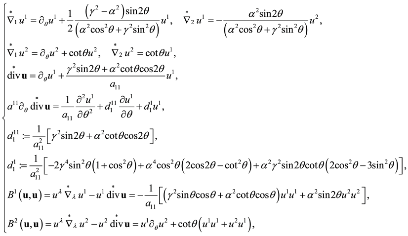
Corresponding metric tensor of  are given by (2.1). We remainder to give the covariant derivatives of the velocity field, Laplace-Betrami operator and trace-Laplace operator. To do this we have to give the first and second kind of Christoffel symbols on the ellipsoid
  as a two dimensional manifolds

Then covariant derivatives of vector  on the two dimensional manifold
 (7.18)
The associated Laplace-Betrami operator on 
 (7.19)
Trace-Laplace operatoe on 

 (7.20)
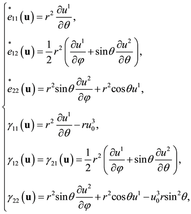
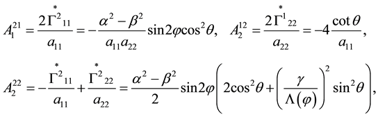
In addition, nonlinear terms
 (7.21)
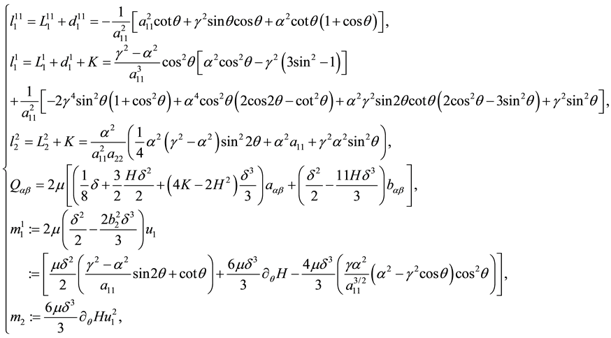
and linear terms
 (7.22)
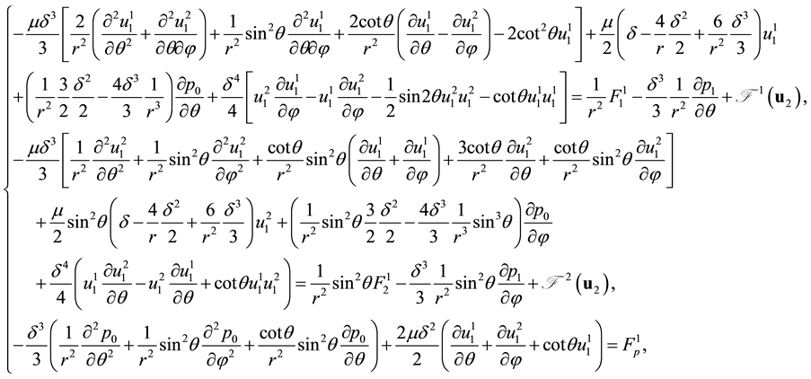
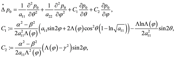
(i) BLE I. Taking (5.1-5.6) and above formula into account we obtain BLE I on the ellipsoid
 (7.23)
where
 (7.24)
 (7.25)
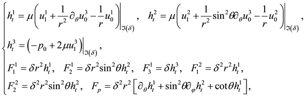
The right terms are given by
 (7.26)
(ii) SEL II. Let consider SEL II given by (5.7) and corresponding variational formulation (5.12) which are followings in semi geodesic coordinate system based on the ellipsoid

(7.27)
where
 (7.28)
 (7.29)
 (7.30)
Calculation of Drag Assume that

 (7.31)
(iii) Axial symmetry Case. If , then boundary layer Equation (7.23) is axial symmetry with
  -axes. Indeed, in this case,
 (7.32)
The covariant derivatives become
 (7.33)
 (7.34)
 (7.35)
Let

Then BLE I (7.23) and SLE II (7.27) become
 (7.36)
where
 (7.37)
The drag is given by
 (7.38)
In the following we concern with the axi-symmetric flow around an ellipsoid, which depends significantly on the Reynolds number and the geometry of the ellipsoid. And the boundary layer equations are solved with spectral method. The fluid approaches the ellipsoid with a uniform free-stream velocity from inlet to outlet. In order to compare with the results in reference conveniently, the results should be dimensionless. Therefore the other parametric equation of ellipsoid is proposed

where  a constant and the parameter
  defines the surface of the spheroid and is related to the axis ratio by
 . A perfect sphere would be represented by
  whereas a flat circular disk would be represented by
 .
.
The Reynolds number based on the focal length, i.e. , varies from 0.1 to 1.0. In the case the
focal length  is the reference length and inlet velocity
  is the reference velocity. Let the total drag coefficient be,

where  is the spheroid projected area. From BLE I the total drag includes two terms and the first term is the pressure part while the second term is the viscous part, i.e.
 , which are defined as,

Therefore the total drag coefficient is also decomposed into pressure and viscous part: , in which,

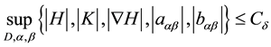
Firstly the numerical solution of boundary layer equations is validated quantitatively by comparison with results in references and finite element method. Table 1 presents results of pressure and total drag coefficients for various Reynolds numbers at . Table 2 presents results of pressure and total drag coefficients for various values of
  at
at . An excellent agreement between the present results and that of Alassar and
Badr [13] are both achieved. And the normal stress tensor  to the supper surface of boundary layer is
considered as the boundary condition of boundary layer equations, which is obtained from the solutions of finite element method. According to Table 1 and Table 2 the precision of drag computation with boundary layer equations is higher than the finite element method, so the boundary layer equations could be used to improve the computation precision of flow in the boundary layer with low cost.
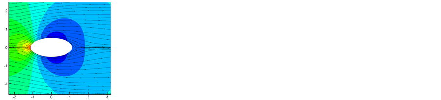
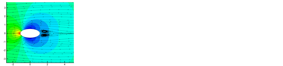
Figure 2 presents the nearly stationary streamline patterns and pressure distributions at different Reynolds numbers 10, 30, 60 and 100 respectively for . Here we note that our streamline patterns are similar to those obtained by Rimon and Cheng [14] for the sphere, since the separation angles and wake lengths are in close agreement with each other. Figure 2(b) shows a clearly visible secondary vortex at
 , in this regard our result is also consistent with Rimon and Cheng’s [14] in spite of the difference in the size of the wake. Furthermore, Figure 2(d) shows a nice structure which corresponds to the a phenomenon observed for the flow around a circular cylinder. Since secondary vortices appear only at relatively high Reynolds number, we may conclude that the wake region is much more active at higher Reynolds number rather than that the wake length has to increase with the Reynolds number.
Figure 3 presents the nearly stationary streamline patterns and pressure distributions at different  0.25, 0.5, 1.0 and 1.5 respectively for
 . As expected, no separation occurs at the low Re values.

 (a) (b)
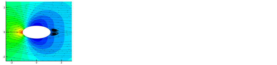
 (c) (d)
Figure 2. Streamlines of the flow:(a) ; (b)
; (b) ; (c)
; (c) ; (d)
; (d)  for
for .
.

Table 1. Comparison of drag coefficients for various Reynolds numbers at .
.
Then the flow details around the trailing edge of ellipsoid for ,
,  are given in Figure 4. It is obvious that the secondary vortex appears in the result of BLE, so more details could be computed by BLE than FEM. Although these flow details is obtained by FEM, its computational cost would be much more expensive than BLE. Let dimensionless pressure be
  and the definition of
  is as follows,
Figure 5 shows shows the surface dimensionless pressure distributions for the case  when
when , 30, 60 and 100. As Re increases, the difference in the pressure between the front and the rear stagnation points increases.
Figure 6 proposes the corresponding pressure distributions in 3D.
 (a) (b)
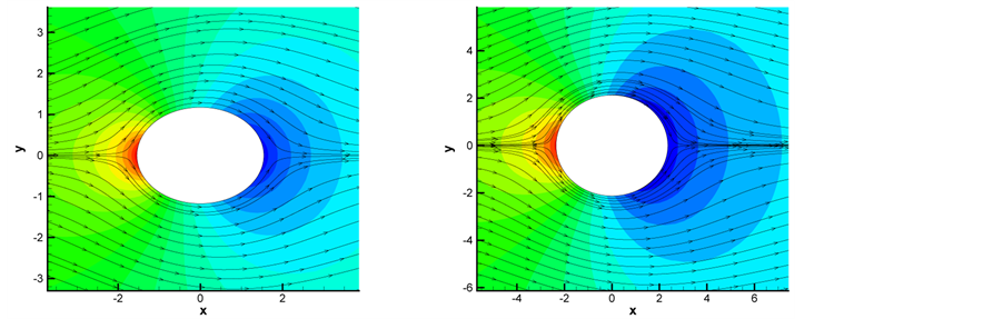 (c) (d)
Figure 3. Streamlines of the flow: (a) ; (b)
; (b) ; (c)
; (c) ; (d)
; (d)  for
for .
.
 (a) (b)
Figure 4. Comparison of flow details for ,
, : (a) FEM; (b) BLE.

Figure 5. Surface pressure distribution for .
.

 (a) (b)
 (c) (d)
Figure 6. Surface pressure distribution in 3D: (a) ; (b)
; (b) ; (c)
; (c) ; (d)
; (d)  for
for .
.
The effect of  on the pressure distribution can be seen in Figure 7. The figure which show the results at
  when
when , 0.5, 1.0 and 1.5 indicates that when
  decreases, a positive pressure gradient may
be expected. The surface pressure distributions are compared between FEM and BLE in Figure 8 for the case  when
when , 0.5, 1.0 and 1.5. The pressure distributions obtained by FEM and BLE are almost the same, however the absolute value of pressure in FEM is generally a little higher than these in BLE, which is consistent with the results in Table 2.
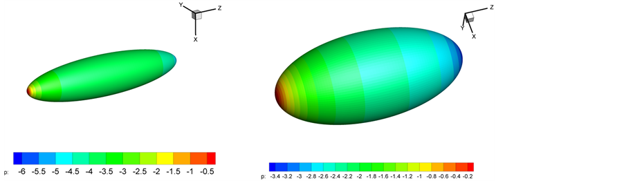
Figure 9 proposes the corresponding pressure distributions in 3D.

Figure 7. Surface pressure distribution for .
.

 (a) (b)
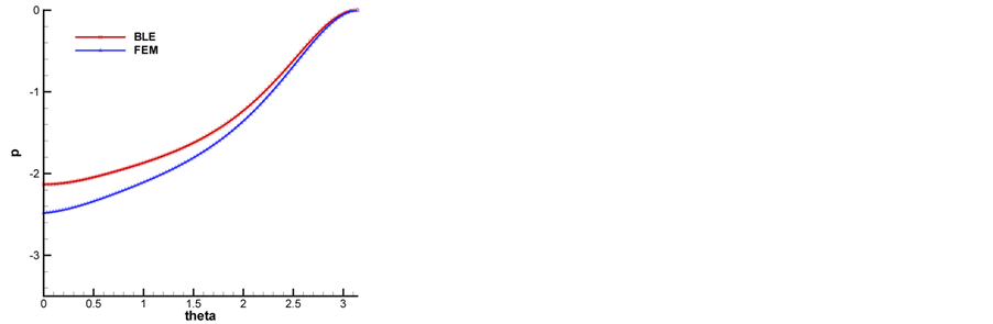
 (c) (d)
Figure 8. Comparison of surface pressure distribution between FEM and BLE: (a) ; (b)
; (b) ; (c)
; (c) ; (d)
; (d)  for
for .
.
 (a) (b)
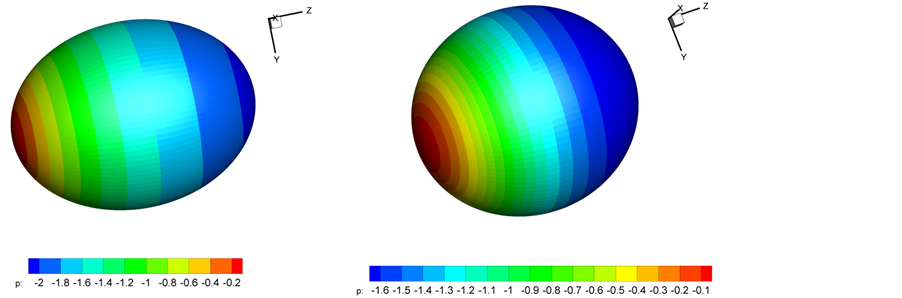 (c) (d)
Figure 9. Surface pressure distribution in 3D: (a) ; (b)
; (b) ; (c)
; (c) ; (d)
; (d)  for
for .
.
Table 2. Comparison of drag coefficients for various values of  at
at .
.
Finally, it has to be emphasized that since flow axisymmetry is assumed in the present study, none of our results give any indication about symmetry-breaking in a real flow. The presented method are, however, not restricted to axi-symmetric flow, the BLE I aforementioned could be used to compute the non-axisymmetric flow.
Support
Supported by Major Research Plan of NSFC (91330116), National Basic Research Program No 2011CB 706505, NSFC 11371288, 11371289.
References
- Li, K.T. and Huang, A.X. (2013) Boundary Shape Control of Navier-Stokes Equations and Dimensional Splitting Methods and Its Applications. Science Press, Beijing (in Chinese).
- Li, K.T., Chen, H. and Yu, J.P. (2013) An New Boundary Layer Equations and Applications to Shape Control. Scientia Sinica (Mathematics), 43, 965-1021 (in Chinese). http://dx.doi.org/10.1360/012012-428
- Li, K.T., Su, J. and Huang, A.X. (2010) Boundary Shape Control of the Navier-Stokes Equations and Applications. Chinese Annals of Mathematics, 31B, 879-920.
- Ciarlet, P.G. (2000) Mathematical Elasticity, Vol. III: Theory of Shells. North-Holland, Amsterdam.
- Li, K.T., Zhang, W.L. and Huang, A.X. (2006) An Asymptotic Analysis Method for the Linearly Shell Theory. Science in China, Series A, 49, 1009-1047.
- Temam, R. and Ziane, M. (1997) Navier-Stokes Equations in Thin Spherical Domains. Contemporary Mathematics, 209, 281-314. http://dx.doi.org/10.1090/conm/209/02772
- Li, K.T., Yu, J.P. and Liu, D.M. (2012) A Differential Geomety Methods for Rational Navier-Stokes Equations with Complex Boundary and Two Scales Paralelell Algorithms. Acta Mathematicae Applicae Sinica, 35, 1-41.
- Li, K.T., Huang, A.X. and Zhang, W.L. (2002) A Dimension Split Method for the 3-D Compressible Navier-Stokes Equations in Turbomachine. Communications in Numerical Methods in Engineering, 18, 1-14.
- Li, K.T. and Liu, D.M. (2009) Dimension Splitting Method for 3D Rotating Compressible Navier-Stokes Equations in the Turbomachinery. International Journal of Numerical Analysis and Modeling, 6, 420-439.
- Li, K.T., Yu, J.P., Shi, F. and Huang, A.X. (2012) Dimension Splitting Method for the Three Dimensional Rotating Navier-Stokes Equations. Acta Mathematicae Applicatae Sinica―English Series, 28, 417-442. http://dx.doi.org/10.1007/s10255-012-0161-7
- Temam, R. (1984) Navier-Stokes Equations, Theorem and Numerical Ananlysis. North Holland, Amsterdam, U.S.A., New York.
- Giraut, V. and Raviart, P.A. (1985) Finite Element Approximation of the Navier-Stokes Equations. Springer-Verlag, Berlin.
- Alassar, R.S. and Badr, H.M. (1999) Oscillating Flow over Oblate Spheroids. Acta Mechanica, 137, 237-254. http://dx.doi.org/10.1007/BF01179212
- Rimon, Y. and Cheng, S.I. (1969) Numerical Solution of a Uniform Flow over a Sphere at Intermediate Reynolds Numbers. Physics of Fluids, 12, 949-959. http://dx.doi.org/10.1063/1.2163685