Open Journal of Fluid Dynamics
Vol.4 No.1(2014), Article ID:44081,5 pages DOI:10.4236/ojfd.2014.41005
Simulation of Average Turbulent Pipe Flow: A Three-Equation Model
Khalid Alammar
Mechanical Engineering Department, King Saud University, Riyadh, KSA
Email: alammar@ksu.edu.sa
Copyright © 2014 by author and Scientific Research Publishing Inc.
This work is licensed under the Creative Commons Attribution International License (CC BY).
http://creativecommons.org/licenses/by/4.0/


Received 16 January 2014; revised 16 February 2014; accepted 23 February 2014
ABSTRACT
The aim of this study is to evaluate a three-equation turbulence model applied to pipe flow. Uncertainty is approximated by comparing with published direct numerical simulation results for fully-developed average pipe flow. The model is based on the Reynolds averaged Navier-Stokes equations. Boussinesq hypothesis is invoked for determining the Reynolds stresses. Three local length scales are solved, based on which the eddy viscosity is calculated. There are two parameters in the model; one accounts for surface roughness and the other is possibly attributed to the fluid. Error in the mean axial velocity and Reynolds stress is found to be negligible.
Keywords:Pipe Flow; Reynolds Stress; Turbulence Modeling

1. Introduction
The problem of turbulence dates back to the days of Claude-Louis Navier and George Gabriel Stokes, as well as others in the early nineteenth century. Searching for its solution, it was a source of great despair for many notably great scientists, including Werner Heisenberg, Horace Lamb, and many others. The complete description of turbulence remains one of the unsolved problems in modern physics. A great deal of early work on turbulence can be found, for example, in Hinze [1] .
Recently, direct numerical simulation (DNS) has emerged as an indispensible tool to tackle turbulence directly, albeit at relatively low Reynolds numbers. Several DNS studies on turbulent flow have been performed recently, including Eggels et al. [2] , Loulou et al. [3] , and Wu and Moin [4] . The latter has carried out DNS on a turbulent pipe flow at Reynolds number of 44,000, which is the largest among the three studies. Mean velocity, Reynolds stresses, and turbulent intensities were presented and discussed, along with visualization of flow structure. Good agreement was attained with the Princeton Superpipe data on mean flow statistics and Lawn’s [5] data on turbulence intensities. Large eddy simulation (LES) is another tool that somewhat bridges between DNS and Reynolds-averaged Navier-Stokes (RANS) methods. In LES, large turbulent structures in the flow field are resolved, while the effect of sub-grid scales (SGS) are modeled. LES investigation, for example, has been carried out by Rudman and Blackburn [6] on a turbulent pipe flow at Reynolds number of 38,000. Mean velocity and Reynolds stresses were presented and discussed, along with visualization of flow structure. Results were reported to compare favorably with measurements.
While DNS and LES are fairly accurate for modeling turbulent flows, they remain limited to relatively low-range Reynolds numbers. This drawback explains the wide-spread of turbulence modeling in industrial applications where the use of DNS techniques remains formidable. Turbulence modeling includes eddy viscosity models which utilize the Boussinesq hypothesis [1] for relating the Reynolds stresses to the average flow field. In turn, the eddy viscosity is determined by using any of a variety of models, including zero, one, and two-equation models, most notably the k-ε. While such models vary in complexity, they share several shortcomings, including isotropy of the eddy viscosity and the lack of generality in wall treatment. Such shortcomings lead to poor results in separated flows and other non-equilibrium turbulent boundary layers [7] .
A second-order turbulence model, which also falls under RANS methods, is the Reynolds stress model. While the model relaxes the isotropic assumption, it remains more complicated with many unknown terms. For more on the subject of turbulence modeling, the reader is referred to, for example, Launder and Spalding [8] .
In this paper, the accuracy of a three-equation turbulence model is assessed. Using the model, average turbulent flow through a pipe is simulated for Reynolds number of 44,000. Uncertainty is approximated by comparing with DNS results of Wu and Moin [4] . Results for fully-developed mean axial velocity and Reynolds stress are presented and discussed.
2. Theory
Starting with the incompressible Navier-Stokes equations in Cartesian index notation, and with Reynolds decomposition, averaging, and following Boussinesq hypothesis, we have
 (1)
(1)
 (2)
(2)
For simplicity, the normal stresses (except for the thermodynamic pressure) and body forces are neglected.  is the eddy viscosity [9] , where
 , and
, and  is a length scale given by
 (3)
(3)
Hence, three local length scales are solved for, based on which the eddy viscosity is calculated. There are three equations for the turbulence length scales with their sources being the average strain rate, along with the molecular viscosity. C1 is a length parameter perhaps attributed to the fluid. C2 is another length parameter attributed to wall roughness.
3. Numerical Procedure
The axisymmetric form of equations (1)-(3) were solved with a finite-volume solver using Gauss-Seidel iterative method, in conjunction with second-order schemes. 20,000 structured cells were used with y+ down to 0.4, Figure 1. The boundary conditions for the length scale were similar to the velocity. Density and viscosity of the fluid were 1000 kg/m3 and , respectively. The inlet velocity was 0.044 m/s. No-slip boundary condition was applied at the wall. The inlet turbulence length scale was set to 1.13e−3 m. C1 and C2 were 8.06e−5 m and 2.93e−9 m, respectively. The pipe diameter was 1.0 m, Figure 2.
4. Results and Discussion
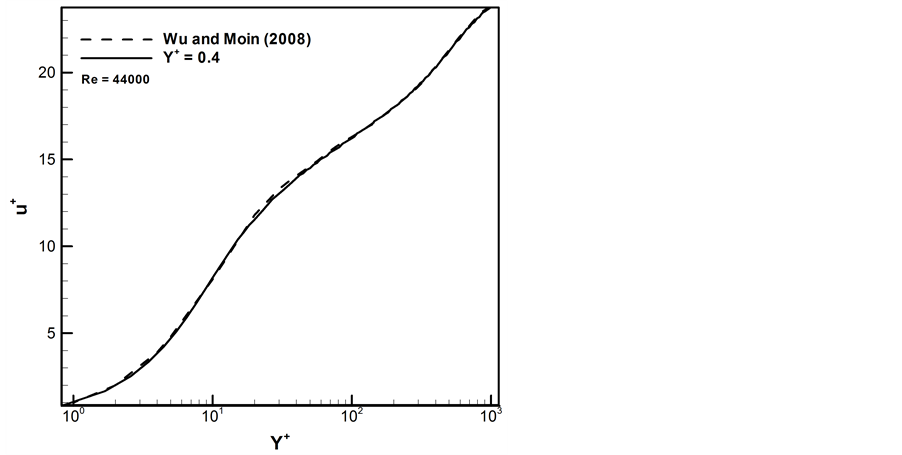
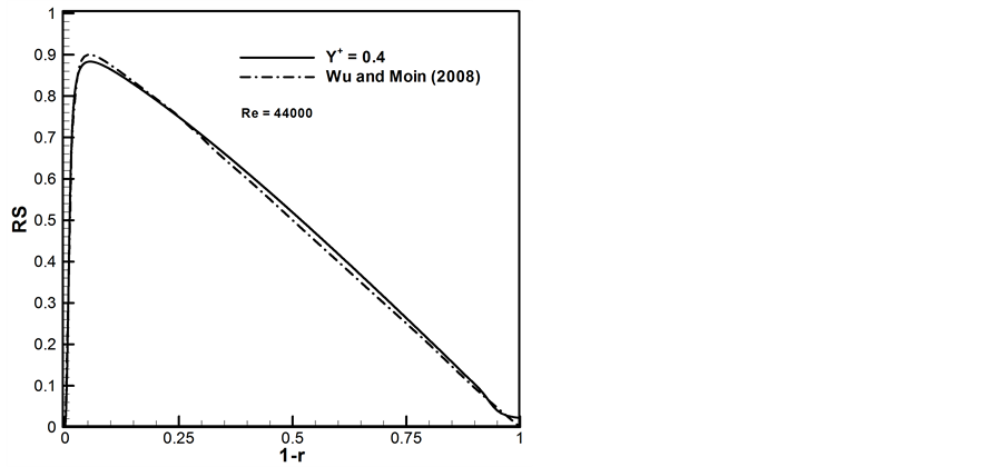
Along with DNS results of Wu and Moin [4] , predicted mean velocity and Reynolds stress distributions are depicted in Figures 3 and 4, respectively for Reynolds number of 44,000. Y+ in this simulation is down to 0.4, which allows for resolving the laminar sub-layer. The agreement is excellent in all regions, including the laminar sub-layer and buffer and outer layers. It’s found that the strain rate in the length equation is responsible for energizing the buffer layer. The predicted friction coefficient was also in excellent agreement with DNS. The constant source term in Equation (3) was observed to shift the velocity profile. It’s proportional to the surface roughness.
5. Conclusion
In this paper, the accuracy of a three-equation turbulence model was assessed. Using the turbulence model, average turbulent flow through a pipe was simulated for Reynolds number of 44,000. Model results for mean axial velocity and Reynolds stress were compared with DNS results. The agreement was excellent. While the model was tested on incompressible axisymmetric flow, testing of the model is needed on more complex flows.

Figure 1. Snap shot of the mesh near the entrance region.
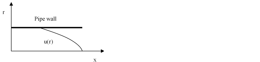
Figure 2. Schematic of the pipe with fully-developed flow.
Acknowledgements
The author would like to extend his sincere appreciation to the Deanship of Scientific Research at King Saud University for its funding of this research through the Research Group Project no RGP-VPP-247.
References
- Hinze, J.O. (1975) Turbulence. McGraw-Hill Publishing Co., New York.
- Eggels, J.G., Unger, F., Weiss, M.H., Westerweel, J., Adrian, R.J., Friedrich, R. and Nieuwstadt, F.T.M. (1993) FullyDeveloped Turbulent Pipe Flow: A Comparison between Direct Numerical Simulation and Experiment. Journal of Fluid Mechanics, 268, 175-209. http://dx.doi.org/10.1017/S002211209400131X
- Loulou, P., Moser, R., Mansour, N. and Cantwell, B. (1997) Direct Simulation of Incompressible Pipe Flow Using a b-Spline Spectral Method. Technical Report TM 110436, NASA-Ames Research Center, Mountain View.
- Wu, X. and Moin, P. (2008) A Direct Numerical Simulation Study on the Mean Velocity Characteristics in Pipe Flow. Journal of Fluid Mechanics, 608, 81-112. http://dx.doi.org/10.1017/S0022112008002085
- Lawn, C.J. (1971) The Determination of the Rate of Dissipation in Turbulent Pipe Flow. Journal of Fluid Mechanics, 48, 477-505. http://dx.doi.org/10.1017/S002211207100171X
- Rudman, M. and Blackburn, H. (1999) Large Eddy Simulation of Turbulent Pipe Flow. 2nd International Conference on CFD in the Minerals and Process Industry, CSIRO, Melbourne, 6-8 December 1999, 503-508.
- Yamamoto, Y., Kunugi, T., Satake, S. and Smolentsev, S. (2008) DNS and k-ε Model Simulation of MHD Turbulent Channel Flows with Heat Transfer. Fusion Engineering and Design, 83, 1309-1312. http://dx.doi.org/10.1016/j.fusengdes.2008.10.001
- Launder, B. and Spalding, D. (1972) Mathematical Models of Turbulence. Academic Press, Waltham.
- Alammar, K. (2008) Turbulence: A New Zero-Equation Model. 7th International Conference on Advancements in Fluid Mechanics, Wessex Institute of Technology, New Forest, 21-23 May 2008, 365-368.
Nomenclature
C: constant, m Ii: unit vector
 : turbulence length scale, m RS: Reynolds stress =
 , Pa U: area-average velocity, m/s u*: friction velocity =
 , m/s
, m/s
 : mean velocity component, m/s u+: normalized mean axial velocity =
xi: Cartesian coordinate, m y+: non-dimensional wall distance = 
 : fluid dynamic viscosity, Pa×s
 : fluid density, kg/m3
w: wall shear stress, Pa