Open Journal of Applied Sciences
Vol.4 No.4(2014), Article ID:44224,13 pages DOI:10.4236/ojapps.2014.44019
World Trade Logics and Measure of Global Inequality: Regional Pattern and Globalization Evolution between 2003-2012
Bruno G. Rüttimann
Swiss Institute for Systems Engineering, Zurich, Switzerland
Email: brunoruettimann@bluewin.ch
Copyright © 2014 by author and Scientific Research Publishing Inc.
This work is licensed under the Creative Commons Attribution International License (CC BY).
http://creativecommons.org/licenses/by/4.0/


Received 31 January 2014; revised 5 March 2014; accepted 12 March 2014
Abstract
The economy is globalizing. But how are the different economic world regions performing regarding globalization of trade flows? Why are they performing differently? Globalization is not only the increase of international trade between certain preferential geographic areas of economy, but also the resulting increase of interweavement of trade flows between different geographical areas, independent of the amount of trade. This paper is a revised and expanded version of the paper entitled “World Trade and Associated Systems Risk of Global Inequality: Empiric Study of Globalization Evolution between 2003-2011 and Regional Pattern Analysis” presented at International Conference on Applied Economics (ICOAE2013), Istanbul, 27-29 June, 2013. This paper analyzes the evolution of world trade flows between 2003-2012 and performs a cross-section analysis of the year 2012. The economic interweavement will be measured by an inequality risk metric applied to the supply-demand matrix. This risk indicator is based on the concept of statistical entropy resulting in an inequality risk measure, giving an indication for the degree of economic globalization and the evolution of globalization in different geographical regions. In addition, it analyses the governing rational of globalization evolution. The result of this research shows that economic trade flows are globalizing, but with clear different regional patterns, not only between globalizing and de-globalizing regions, but also within the globalizing and de-globalizing regions itself. The emerging economies such as China or the Middle East are globalizing whereas mature economies such as North America and Europe are de-globalizing, confirming for globalization of the inverse Kuznets evolution. The different patterns between the different economic world regions can be explained by using the Globalization Type’s Model as well as the Central Theorem of Globalization.
Keywords
Globalization; Risk Metric; Inequality; Measure; Entropy; Trade Flows; Pigou-Dalton; Kuznets; Heckscher-Ohlin; Linder; Globalization Types; Central Theorem

1. Introduction
Globalization is a natural phenomenon of an open economic system. Liberalization and deregulation of trade barriers as well as bilateral economic development agreement have been leading to an increase in trade and therefore in wealth generation, and also bear the danger of exploitation of disadvantaged regions. The emerging economies, namely the BRIC countries (Brazil, Russia, India, China), will be the major drivers and stakeholders in the future importance of economic development. Within the emerging economies, substantial differences within action scope or preferential trade partners are observable. The development of economic globalization is a mix of increase in physical trade, sustained foreign direct investments, and an increase in human mobility, all supported by telecommunication and increase in transparency of efficient market places via the world wide web. Different types of indicators have been developed to measure the multiple dimensions of globalization. The evolution of world economic development is monitored by the WTO (World Trade Association) as well as e.g. the yearly published KOF globalization indicator (Konjunktur-Forschungsstelle) of Swiss ETH (Eidgenössische Technische Hochschule).
In this updated study, we will concentrate the analysis first on the evolution of physical trade flows within the major world economic areas given by the WTO table i04, namely North America NA, South Central America SCA, Europe EU, Commonwealth of Independent States CIS, Africa, Middle East ME, and Asia. We will apply an inequality indicator based on statistical entropy which incorporates also the intrinsic reason of minimizing risk by even distribution of portfolio, formalizing a built-in rational explanation of globalization [1] . Within the main economic globalization types, namely type 1 (physical flow globalization), type 2 (financial and capital globalization), type 3 (human factor globalization, i.e. migration and services), each is characterized by subtypes [1] -[3] of this comprehensive globalization model. We will use the type 1 globalization to explain the different evolution of globalization in each geographical region.
Second we will apply the Central Theorem of Globalization (CTG) and its corollary [1] [4] to understand the underlying logic of evolution of trade. The paper will investigate questions such as: how are different globalization patterns linked to the trade flows? Why should different regions perform differently? Is it a consequence of different resource endowment or the maturity of the economy? Which are the possible economic driving causes for the different trade patterns?
2. Theoretical Background
In the following, we will apply the globalization measure according to [1] [4] to foreign trade flows. From the paradigmatic interpretation of thermodynamic entropy we can define risk as a dualistic view of order in an economic system, therefore the more order (i.e. inequality) that exists in an economic system the more risky the economic system (or vice versa, the more equality a system shows the less risk it presents). The greater the inequality compared to the riskless state with equality yXY = 1, the larger the risk of an atomic element. Whereas in the here presented context inequality refers rather to a single element of a system, the concept of risk can be aggregated to the entire system.
2.1. Risk as a Measure for Globalization
According to the Pigou-Dalton Transfer Principle and the interpretation of entropy law, we will apply the Minimum Risk Principle [1] [4] to analyze the foreign trade i.e. the material globalization type 1 [1] [2] dealing with physical flows of a product a, applying to which country X exports to which countries Y, and which country imports from which countries represented by the trade matrix Ta = [taXY]. For a trade system we can build the market share vector of an economy and calculate the inequality measure yXY as the market share of X in Y compared to the overall market share of X. For economy X we can calculate the risk rX(yXY) of its portfolio of activities in the countries Y. The lower the inequalities in each country Y the lower the risk value and therefore the higher the globalization degree of the country X. If the inequality is yXY = 1 for all Y then country X has the same market share in all countries Y and its portfolio of trade-flows is proportional to the market composition according to its competitiveness. We can consider the CTG and its corollary as the basics to explain that our economy will globalize naturally with the existing deregulation tendency. This risk metric is a genotypic measure, bearing the intrinsic law of economic globalization.
2.2. Maximizing Value Net of Risk
But entropy is not the sole governing physical law of thermodynamics. Indeed, if a transformation happens is determined by free enthalpy. The same is also applicable to economics [1] . By adding the concept of thermodynamic enthalpy to the economic system, we can also explain the presence of an eventual de-globalization trend (i.e. an increased order of the economic system corresponding to an increased inherent economic risk of the system). This matches the fundamental economic law that a higher risk corresponds generally to a higher return.
Minimizing risk is only one cardinal law (this law models the globalization extension), maximizing profit is the other cardinal one (this law models the final rational acting). Globalization is extending the business scope to new geographic areas, and the aim is
• to increase the profit generation (explicit strategy of profit maximization), and at the same time;
• it reduces the risk of the portfolio (implicit law of risk minimization).
The final governing principle of economic globalization is therefore risk deducted value maximization [1] [4] . With this principle we can explain the rational of any economic actor not only limited to perfect competition models but including oligopolistic markets comprising MNE (Multi National Enterprises) and extended to world trade why globalization happens.
3. Methodological Approach
To measure the globalization degree of the set of geographical regions, defind at the beginning, regarding the economic dimension of trade, as well as the evolution of globalization, we will use the inequality risk metric [1] [4] . This metric represents a paradigmatic approach of Boltzmann entropy of a thermodynamic system leading to statistical entropy. Instead of talking about entropy in economics, in the following we prefer to talk about risk of an economic system, which is more appropriate, i.e. the higher the entropy, the lower the risk of the economic system, i.e. the higher the globalization degree.
Let us define the trade matrix Ta = [taXY] showing the trade flows from economic region X to economic region Y for a product a or, in this case, for the whole trade volume. We can now build the market share array of an economic region and calculate the inequality measure yXY = pXY/pX as the market share of X in Y compared to the overall market share of X obtaining the inequality matrix for the whole economic system ya = [yaXY]∞. For economy X we can calculate the risk rX(yXY) of its portfolio of activities in the countries Y as the 2nd momentum of the elements belonging to the inequality array yX relative to the attractor 1
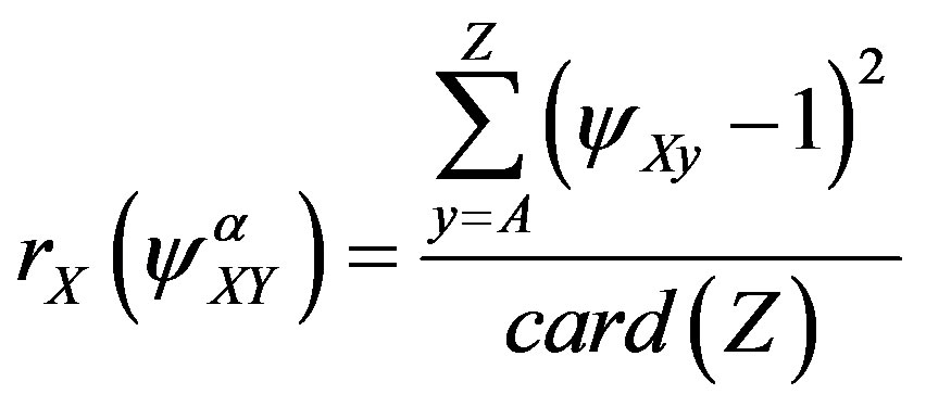 (1)
(1)
The lower the inequalities in each country Y of supplying country X, i.e. the more even is the repartition of trade portfolio and therefore the interweavement with other economies, the lower the aggregated risk value and therefore the higher the globalization degree of the country X; this concept leads to the CTG and its corollary [1] [4] [5] , which we will apply. If the inequality is yXY = 1 for all Y then country X has the same market share in all countries Y and its portfolio of trade-flows is proportional to the market composition and marginal matrix distribution according to its competitiveness and the inequality risk rX(yXY) will become 0, i.e. attain maximum globalization. The array rX(yXY), containing the single risk of each economy, can be aggregated to the risk of the entire system of economies r(yXY) representing the world globalization degree in terms of interweavement. Inequality measure can be applied to supply or demand; we will analyse in the following for the pattern analysis rather the supply-side, i.e. the exports marginal distribution of the trade matrix. The aggregated world risk value, of course, is the same for both marginal distributions. We will interpret empirically the resulting patterns based on theoretical considerations.
The upper part of Table 1 shows the world trade flow matrix of the year 2012 (source WTO Table i04), as well as in the middle part, derived trade shares measures of the geographic regions, and in the lower part relative inequalities calculated according to [1] [4] . The single inequalities are then aggregated to a risk measure of each economic region according to the two dimensions of supply portfolio (exports) and demand structure (imports); the matrix contains also geographic intra-trade tXX. These individual “geographic” risk figures rX(yXY) for ex

Table 1. World trade matrix (in b$) with inequalities and risk measures for 2012.
ports, and rY(yXY) for imports, are finally aggregated to the world risk index r(yXY) measuring the economic globalization degree, i.e. the extension of the world economic trade system.
4. Analysis of Trade Evolution and Globalization
The world trade flows on an aggregated level have increased according to WTO source from 7290 b$ in 2003 to 17,563 b$ in 2012 showing the unrelenting growth of the world economy with a deep throwback to 11,978 b$ during the world financial crisis in 2009, as shown in the data in the upper part of Table 2. The associated geographical areas and world risks, calculated according to Equation (1), are shown in the lower part of the same Table 2; it emerges that economic world risk metric diminished from 4.43 in 2003 to 1.62 in 2012 demonstrating increased interweavement of economies, hence a more globalised world of trade flows. The graphical evolution of regional risks is presented also in Figure 1 and reveals a heterogeneous evolution.
Building the correlation between world trade and world supply risk we obtain the regression model shown in Figure 2. The applied model is the model calculated using figures from 2003-2009 presented in [5] but with the figures from 2010, 2011, and 2012 added to test the model. The present results including the three recent years confirm the validity of the regression model and already emerged results from the 2003-2009 analysis [5] . It shows, that the risk level diminishes, i.e. the interweavement of globalization increases with the growth of trade volume. On the contrary, the risk increases with shrinking trade volume; that means, that during an economic downswing exports are concentrated on specific preferential areas less affected by the downswing, increasing portfolio inequality and therefore increasing risk level.
If we look at disaggregated data, i.e. at the evolution of regional risk shown in the lower part of Table 2 or Figure 1, we notice that Asia and SCA have shown a continuous reduction in risk, also during 2009, i.e. a clear globalization trend, whereas NA, and especially EU, have shown a continuous de-globalization trend during the period 2003-2012 (Figure 1) but NA with a significant through-back in 2012. The regions CIS and ME show also a globalization tendency but suffered a throwback in 2009 due to the world economic crisis. This might be given by their heavy commodity orientation: commodities being very sensitive to economic cycles, standing at the top of the value chain. Also Africa showed the same throwback as CIS and ME but after 2009 has continued to increase its risk level; this is an indication that the trade flows were redirected and concentrated. Indeed, ship
Table 2. Evolution of supplies and risks during 2003-2012 for different macro-economic regions.
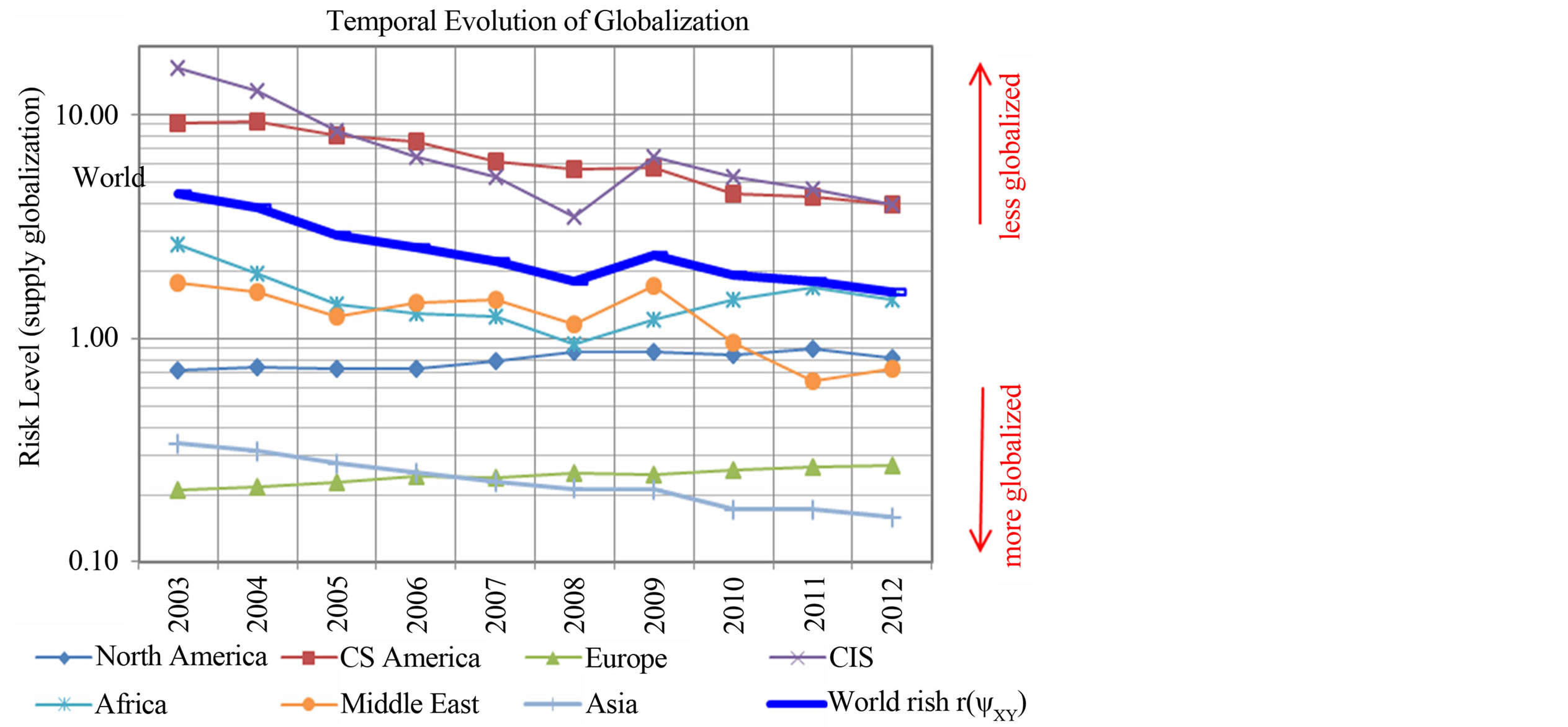
Figure 1. Regional risks of different macro-economic regions according to Table 2 revealing heterogeneous evolution.
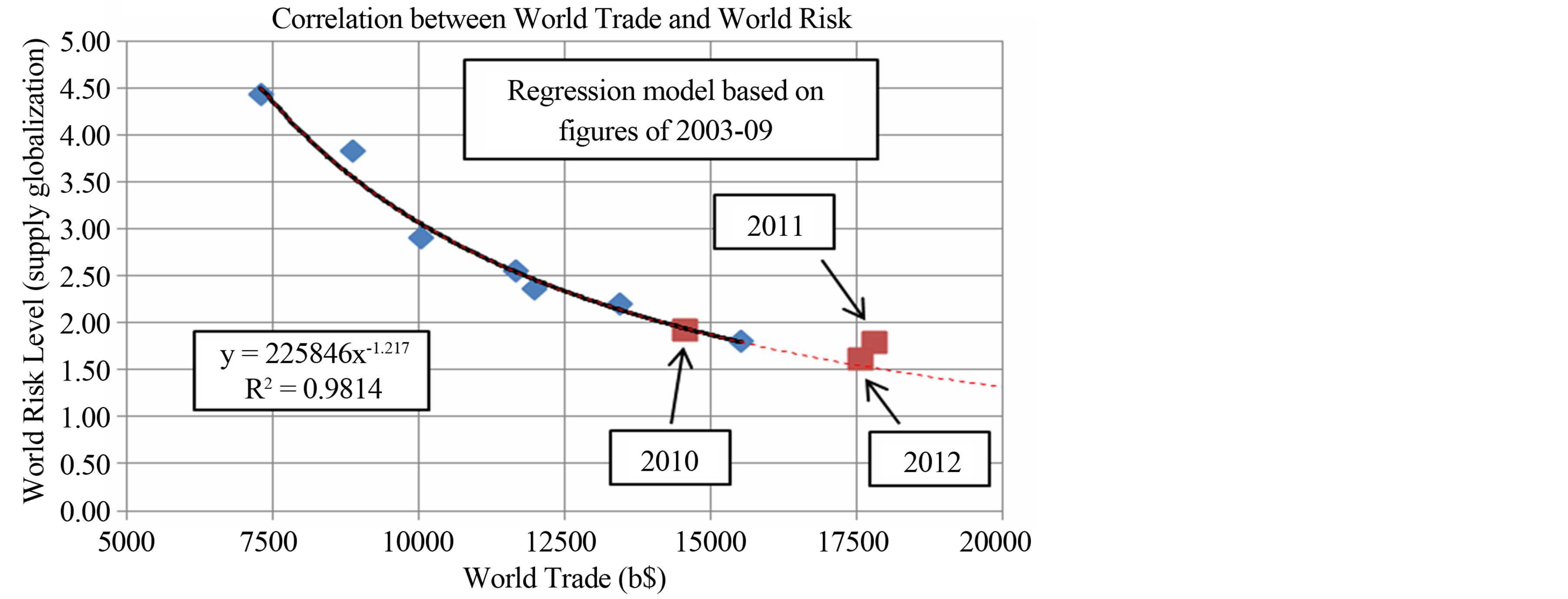
Figure 2. Modeling on aggregate level.
ments from Africa to Europe and Asia have increased over-proportionally (this data has not been annexed to the paper). In 2012, Africa increased trade further but with different composition and reduced its risk level.
Plotting the data from Table 2 regarding the different macro-economic geographical regions on a scatterplot, we obtain Figure 3 revealing the comparative evolution of globalization in the different geographic areas with increasing trade flows. The enveloping curve shows a similar pattern as the aggregated data in Figure 2, i.e. diminishing risk with growing trade volume. Nevertheless, whereas most regions are increasing global interweavement (diminishing their risk level) with growing trade volumes, it is observable that Europe has steadily increased its risk level with growing trade volume from 0.21 in 2003 to 0.27 in 2012 and North America even more, from 0.71 to 0.90 in 2011 (leaving apart for the moment the value 0.81 of 2012), i.e. an antithetic evolution. We can therefore not generally state that increased trade volume is increasing global interweavement. Why this difference? Have we to expect the same evolution on an aggregated level with further increasing trade flows, i.e. substituting the L-shaped curve with a U-shaped curve with polynomial modeling?
Analyzing the difference in globalization evolution in different geographical regions, comparing CAGR of trade and CAGR of supply risk according to Figure 4, we notice that there emerge two clusters: one with the advanced economies EU and NA and another with the emerging economies. The clusters of globalizing countries (SCA, CIS, ME, Africa, Asia) are characterized by high growth rates of trade whereas the de-globalizing countries (EU and NA) are characterized by reduced growth rates of trade; i.e. the segregation of pattern is not

Figure 3. Regional pattern on disaggregated level.

Figure 4. Emerging clusters of macro-economic regions.
given by the absolute volume of trade but on the growth rate of trade. It is the growth rate which will determine if an economy is globalizing or de-globalizing.
If we consider also the demand risk of an economical region, i.e. inequality in imports, we obtain the overall globalization evolution shown in Figure 5. From Figure 5 and Table 1 it emerges that EU is the most globalized region from a sourcing view point with a demand risk rY(yXY) of 0.34 followed by Asia with 0.36 and ME with 0.37. The overall most globalized region, according to Pareto iso-risk curves, is Asia, followed by EU and ME, i.e. reflecting mainly supply risk; we will continue therefore to concentrate on this dimension.
High risk level, i.e. high inequality, usually originates from predominant autarchic economy orientation with limited foreign trade. This is typical for emerging economies as well as for geographically isolated economies, such as SCA, or politically isolated economies, such as CIS, which focus on the home market. Low risk level, i.e. high globalization of trade, is seen in economies such as Asia, EU and ME. According to Table 1, also in 2012 ME showed with 0.73 a lower supply risk level than NA with 0.81, i.e. ME remains more globalized than NA.
Figures 6 and 7 show the behavior of globalization during the recession of an economic cycle. Figure 6
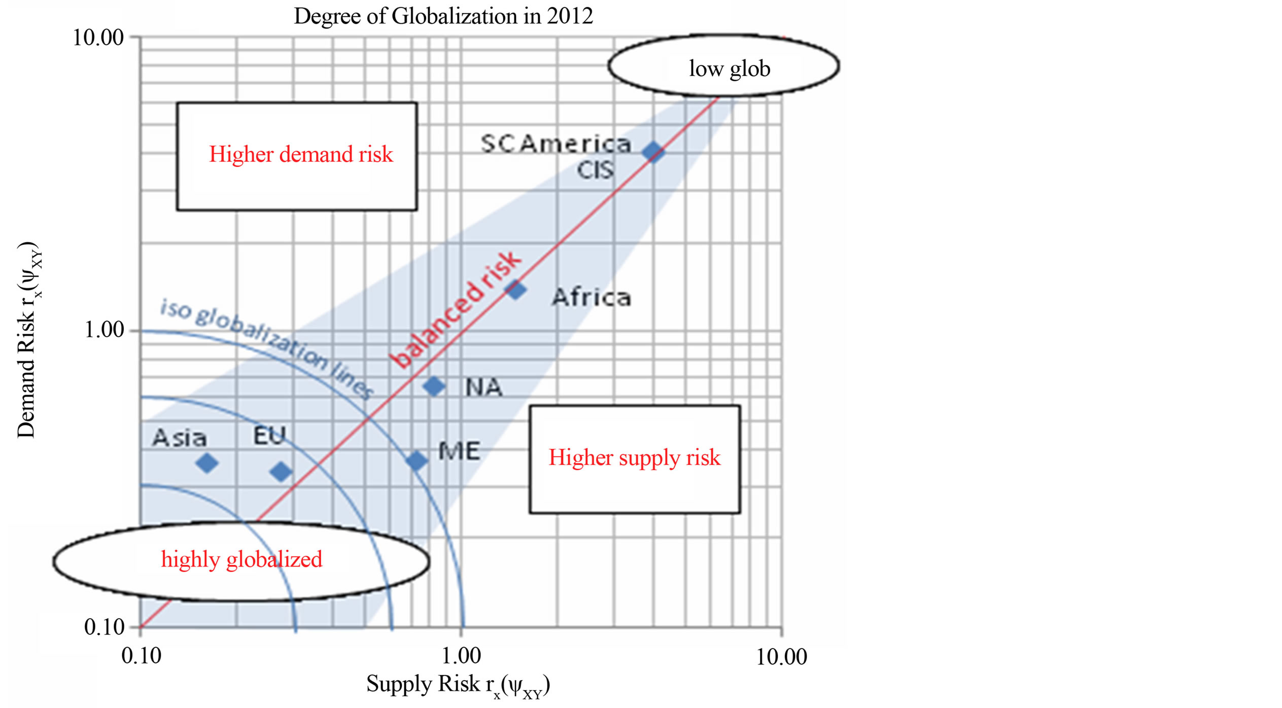
Figure 5. Most globalized regions.
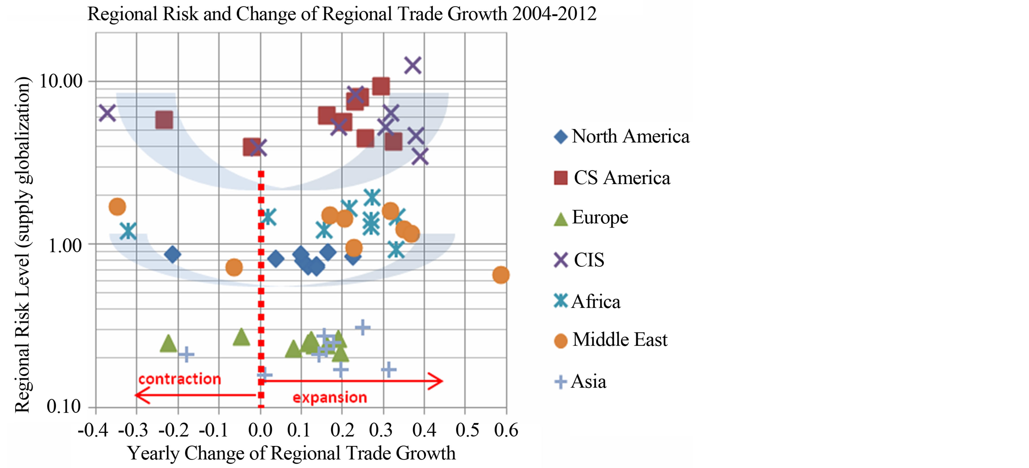
Figure 6. Evolution of regional risk during economic cycle.
shows that risk level is increasing during a contraction of trade also on a disaggregated level as the model in Figure 2 shows. In addition, Figure 7 shows that there are different sensitivities in risk change of the different economic regions. Economic regions well endowed with commodities such as CIS, ME, and Africa show a coherent behavior of high sensitivity, whereas mature economies such as NA and EU show no relevant change in globalization levels during economic cycles. Only SCA behaved differently with low sensitivity; this shows that there are also other driving factors influencing risk change than merely change in economic cycle, such as a well balanced portfolio composition of destination countries for export giving more robust solutions.
5. Interpretation of Results
The question arises what are the causes of this different evolution in globalization? From empirical interpretation there are possibly two main causes which drive the different evolutions of trade globalization:
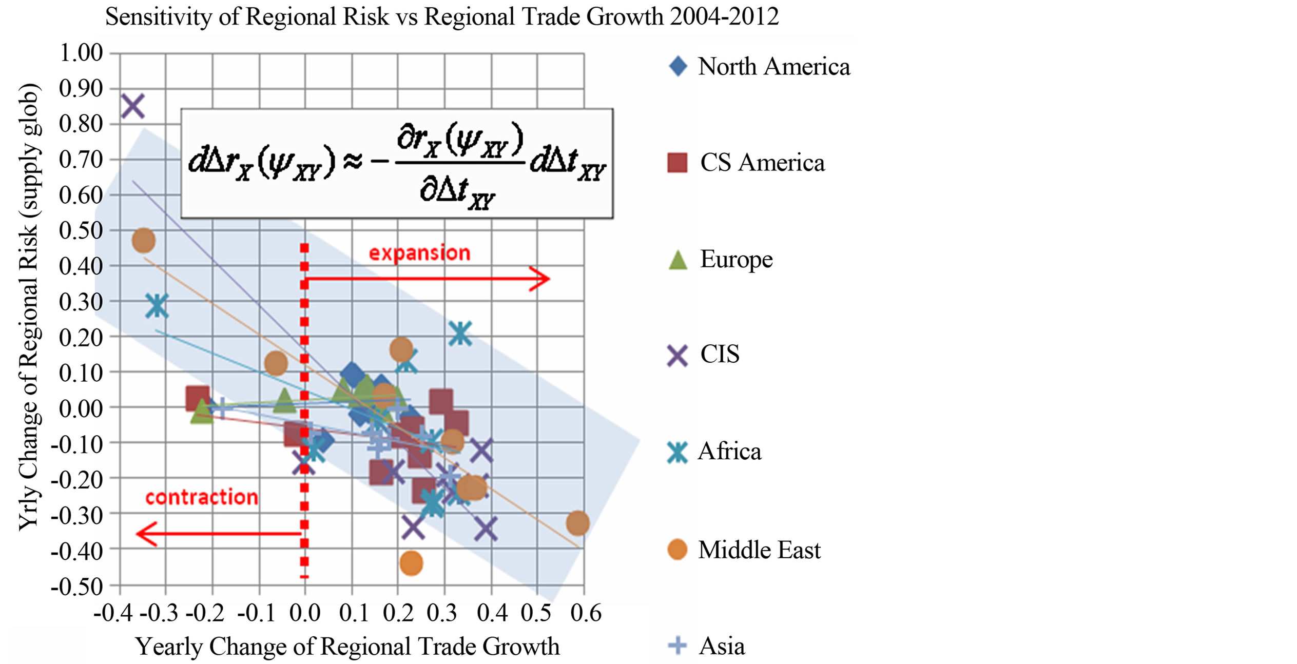
Figure 7. Sensitivity of regional risk during economic cycle.
• The maturity degree of economic region (advanced or emerging);
• The characteristics of product/goods (commodities or specialties, as well as low-cost products).
Indeed, the product characteristics determine the business type (commodities, standards, specialties, convenience) and the related globalization types with its specific logic [1] -[3] . We will concentrate on the three subtypes of type 1 trade globalization: type 1a the globalization of commodities, type 1b the globalization of specialties, and type 1c the opportunistic low-cost globalization. Figure 8 shows synoptically the difference between the three subtypes of trade globalization. We have to be aware that globalization types may overlap, e.g. capital globalization type 2a with trade type 1b or type 1c; these globalization types, each with different logics, give a rough classification to facilitate understanding of globalization [1] . Let us give in the following a brief overview; for detailed information we refer to [1] , as well as [2] , and [3] entering into all three main types of economic globalization as well as their seven sub-types.
Type 1a is the globalization of commodities with unidirectional flows tod from the country of origin O to the industry countries of destination D. The main drivers for this type of globalization are shown in Equation (2); these are the demand Vd for a certain commodity in the industrial country and the price pr of the commodity which is determined by the demand/offer at efficient commodity exchanges, as well as the substitute materials and their prices ps and the production cost Po in the country of origin.
 (2)
(2)
Type 1b is the globalization of specialties characterized by bidirectional trade flows tAB between countries A and B modeled with Equation (3). The main drivers for that type of globalization are: the volume demand VA and VB for the product in the producing country A and the demanding countries B, as well as market growth rates gA and gB, their prices pA and pB for the products produced in A and B, as well as the comparative product characteristics παβ and prices between similar products; for detailed explanation see [1] [5] . Due to the differentiation possibilities of the products, the price fixing is made from the view of the value for the customer and competitive marketing decisions.
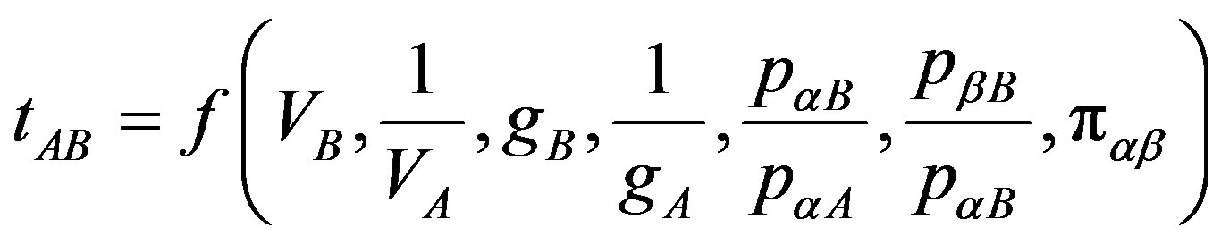
 (3)
(3)
Type 1c is a transient globalization type with unidirectional trade flows tZK from the low-cost country Z to the high-price countries K and is based on exploiting the structural advantage of production cost ΔpZK, as shown in
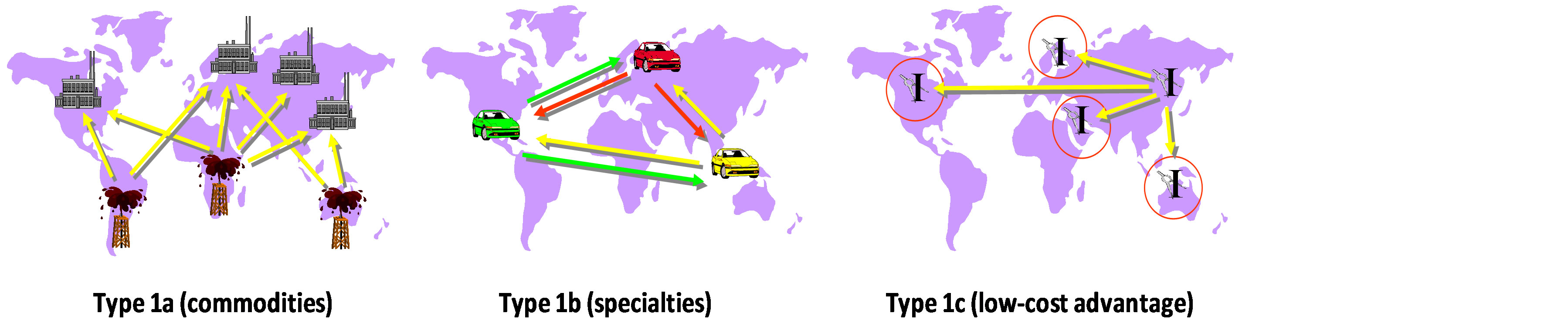
Figure 8. The three subtypes of trade globalization (type 1 globalization).
Equation (4). The trade flows depend also on the capacity filling situation in the low-cost country (PZ/VZ) and how attractive the price differences (pK/pZ) are. This type of globalization is a transient type, existing as long as the opportunities are intact. Low-cost countries are e.g. the BRIC countries. Due to the different stages of maturity of the BRIC economies, this type will last for long [6] .
 (4)
(4)
These Functional relations (2), (3), and (4) are based on empirical as well as theoretical considerations; they are derived from proven basic economic laws. The three different equations show that globalization is not equal to globalization; different driving logics govern the triggering and evolution of globalization leading to different trade globalization patterns. Giving insights to the transaction mechanism, they allow, together with the globalization types 2 and 3, to explain on macro-economic level the transaction evolution, in order to model competitive behavior and potential evolution of value chains [7] -[9] . It has to be mentioned that the Equations (2)-(4) are not state equations as generally used in neo-classic economy for modeling equilibrium, but they are functional relations modeling the triggering and transition from one state to the other, i.e. the dynamic aspect of evolution.
With that in mind, let us analyze the products of trade. In Table 3 [10] are shown the export flows of main economic regions by product family divided in manufactured products, fuels and mining products, as well as agricultural products. The industry logic of manufactured products follows globalization type 1b and 1c, whereas the logic of fuels and mining trade flows are governed by globalization type 1a; basic agricultural commodities follow also type 1a globalization.
If we compare the information in Table 3 with the globalization evolution of different world regions in Figure 3, we can empirically draw the chart of Figure 9 (adapted from [10] ), where we put the type of globalization on the evolution of globalization. This shows inverse Kuznets evolution, i.e. with decreasing inequality at the beginning and then, in mature advanced economic status, again with increasing inequality due to concentrated preferential trades. It shows that type 1a stands at the beginning of globalization evolution, followed by absolute cost-advantage and differentiated products in the evolution of an emerging economy. The rational of interpretation makes sense; indeed, emerging economies do not yet have developed technology to sell, but are often endowed with raw material to be extracted and shipped all over the world, increasing with that their globalization with sinking risk indicator according to type 1a globalization logic (Heckscher-Ohlin’s endowment pattern model). Preferential export destinations may increase risk indicator again, as is the case with African exports (see Figure 2, period 2009-2011). Emerging economies can also benefit from low wages and have therefore an advantageous cost-structure to produce intermediates or low-technology products for export increasing globalization following the opportunistic low-cost type 1c globalization logic. Low-cost products are appealing for every economy and fuel therefore opportunistic type 1c globalization. Production of differentiated specialty products allow the development of further exports and are further fuelling globalization governed by the type 1b globalization logic. After the initial 360˚ export orientation approach, mature economies will also install preferential destinations. This is given by the fact that similar (advanced) economies are more likely to have trade together than complementary economies (Linder’s demand pattern model). Another deriving reason is, that trade partners are selected on economic return considerations and ethical business practices, which will invert the globalization tendency in terms of trade interweavement, concentrating commerce to selected destinations with bilateral trade agreements.
Nevertheless, the globalization type model explains the phenotypic dimension of trade, based on different business types such as commodities, specialties, standards, and convenience goods and their pertinent forms of
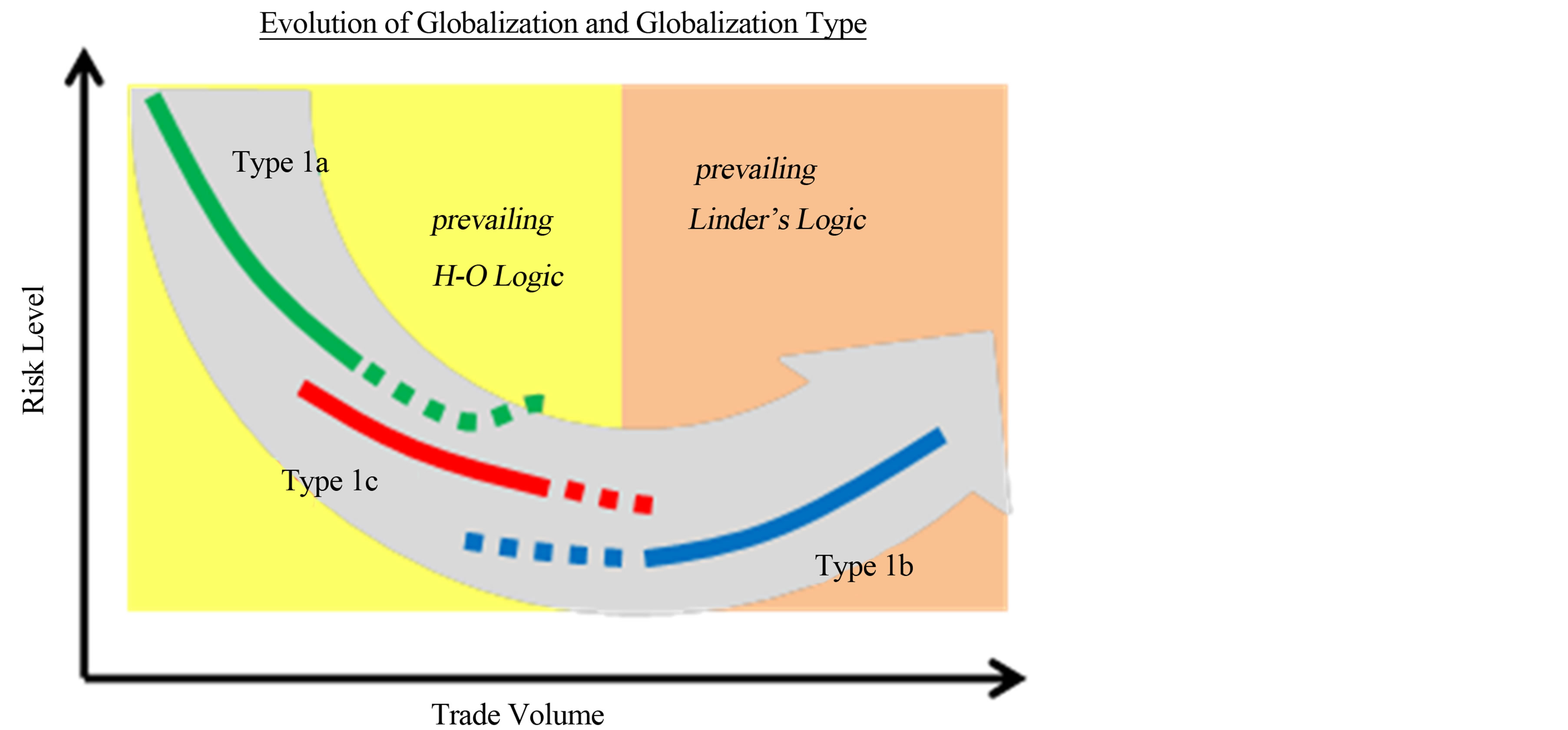
Figure 9. Resulting empiric model of globalization evolution.
Table 3. Regional exports and relative main globalization types.
globalization with its underlying rational [1] -[3] [7] -[9] . It does not fully explain why we observe at the same time globalization (decrease of risk level) and de-globalization (increase of risk level) within the same economic area. Indeed, NA e.g. experienced in 2012 a significant increase in globalization reducing its risk level from 0.90 in 2011 to 0.81 in 2012, against the trend observed since 2003 (see Figure 1). On the other hand, EU reduced further its globalization level increasing its risk indicator from 0.26 in 2011 to 0.27 in 2012, continuing its steady de-globalization trend (N.B. risk value is still on a very low level documenting a very high trade interweavement with other regions, i.e. globalization, compared to other economic regions). This is partly due to the increase of trade for NA and the decrease in trade for EU (according to the aggregate modeling, see Figure 2) but also for a more balanced export pattern for NA, finding new opportunities. The question arises, why certain countries or economic regions, i.e. the aggregation of economic actors, concentrate their trade on preferential destinations taking, deliberately or unintentionally, de-globalization, i.e. a higher risk, into account? Apart from Linder’s demand pattern model and the inverse Kuznets type globalization evolution combined with the globalizations types model (Figure 9) there is a dualistic explanation.
Indeed, globalization can also be explained by the Minimum Risk Principle, derived from portfolio theory, and the CTG [1] [4] . Apart from conjuncture-influenced structural change of the marginal distribution of the trade matrix, changing also inequality measures, economic policies are driven by maximizing profit. Maximizing profit means exploiting competitive advantages in areas where the products show a demand. This leads to abandon the Minimum Risk Principle exporting to all over the world and to concentrate flows, according to Linder’s demand pattern model, to preferential destinations, following the Maximizing-Value-Net-of-Risk Principle [1] [4] , which can be assimilated to free enthalpy of a thermodynamic system. The paradigm to assimilate an economic system, composed of many economic actors, to a thermodynamic system, composed of many physics molecules, might be only approximate right; indeed molecules follow exact physics law whereas economic actors, even if they should behave like the “homo oeconomicus”, they only can be considered in the average to be rational. Nevertheless, the average rational acting of economic actors leads to have trade with preferential economic partners in defind geographic regions, leading finally to de-globalization, measured as interweavement of trade flows, despite trade volume is increasing. This is why EU since 2003, and perhaps even before, shows a steady de-globalization trend.
6. Findings and Conclusions
Based on the results of this empiric based analysis we can summarize the following findings about economic globalization, seen as interweavement of trade flows, giving increased insights into this globalization phenomenon:
• At the first stage, world economic globalization at aggregate level of all economies is correlated to trade volume (L-curve): increased trade will reduce risk level (increased globalization);
• The economic world as a whole is globalizing but with different evolutions for the different economic regions: globalizing for the emerging economies, de-globalizing for the mature economies;
• This means that for each economic region, as the maturity degree of an economic region evolves, we can see the transformation from an L-shaped curve to an U-shaped curve, i.e. inverse Kuznets pattern;
• Further, graphical correlation shows: not the trade volume but the growth rate determines the evolution of globalization;
• In addition, the structural segregation of de-globalizing advanced economies from globalizing emerging economies is not given by trade volume but by reduced trade growth, i.e. the reduced growth rate of production leads to de-globalization;
• Emerging economies, mainly focusing on commodities, are more sensitive to volatility and therefore to de-globalization as they respond to economic cycle contraction then advanced economies, advanced economies which maintain their risk level, i.e. their globalization degree;
• A strong globalization tendency is initially seen by economies following commodity type 1a globalization and subsequently low-cost opportunistic type 1c globalization following Heckscher-Ohlin theory. Specialty type 1b globalization, observable more in advanced economies, favors de-globalization, due to preferential destinations according to Linder’s theory;
• The evolution of globalization (measured as interweavement) given by the CTG can be explained by the universal ultimate economic rational Maximizing-Value-Net-of-Risk logic, corresponding to the efficient frontier of a portfolio of activities, which also allows explaining a de-globalization evolution.
These are the confirmed and enlarged findings regarding to [10] to explain the comparative differences of globalization evolution for the different macro-economic geographical regions, giving an increased understanding of globalization phenomenon. The evolution has to be monitored during the next years to verify these findings.
References
- Ruettimann, B. (2007) Modeling Economic Globalization—A Post-Neoclassic View on Foreign Trade and Competition. Verlagshaus Monsenstein und Vannerdat OHG, Münster.
- Ruettimann, B. (2009) Modelling Economic Globalization—The Basic Globalization Types. Global Studies Association Conference, Royal Holloway University, London.
- Ruettimann, B. (2011) A Comprehensive Globalization Model to Analyze Industry Logics: The Seven Economic Globalization Types. International Conference on Applied Economics 2011, Perugia, 7 October 2011.
- Ruettimann, B. (2011) An Entropy-Based Inequality Risk Metric to Measure Economic Globalization, Elsevier Procedia Environmental Sciences. Procedia Environmental Sciences, 3, 38-43. http://dx.doi.org/10.1016/j.proenv.2011.02.008
- Ruettimann, B. (2012) Measuring Spatial Extension of Economic Globalization. International Conference on Applied Economics 2011, Perugia, 7 October 2011, 509-517.
- Rüttimann, B. (2011) Werden die chinesischen Halbzeugexporte die Märkte überfluten? DOW JONES NE Metalle Monitor, No. 1, Dow Jones News.
- Rüttimann, B. (2008) Which Globalization for the Aluminium Industry—A Normative Analysis Exploring Alternative Business Models. ALUMINIUM, 84 1/2-2008, 16-22, 3-2008, 14-21, Giesel Verlag.
- Rüttimann, B. (2008) Which Globalization for the Aluminium Industry. Proceedings of the ALUMINIUM 2008 Congress, Essen, 23-25 September 2008.
- Rüttimann, B. (2010) Globalisierung verstehen heisst Märkte beherrschen—Wie man durch Analyse der Geschäftsund Industrielogik ein normatives Modell der Globalisierungsformen erhält. iO New Management, Springer Verlag, Berlin.
- Rüttimann, B. (2013) World Trade and Associated Systems Risk of Global Inequality: Empiric Study of Globalization Evolution between 2003-2011 and Regional Pattern Analysis. Procedia Economics and Finance, 5, 647-656. http://dx.doi.org/10.1016/S2212-5671(13)00076-2