Advances in Linear Algebra & Matrix Theory
Vol.4 No.2(2014), Article
ID:46828,9
pages
DOI:10.4236/alamt.2014.42008
Numerical Quadratures Using the Interpolation Method of Hurwitz-Radon Matrices
Dariusz Jacek Jakóbczak
Department of Computer Science and Management, Faculty of Electronics and Informatics, Technical University of Koszalin, Koszalin, Poland
Email: dariusz.jakobczak@tu.koszalin.pl
Copyright © 2014 by author and Scientific Research Publishing Inc.
This work is licensed under the Creative Commons Attribution International License (CC BY).
http://creativecommons.org/licenses/by/4.0/


Received 11 April 2014; revised 12 May 2014; accepted 19 May 2014
ABSTRACT
Mathematics and computer sciences need suitable methods for numerical calculations of integrals. Classical methods, based on polynomial interpolation, have many weak sides: they are useless to interpolate the function that fails to be differentiable at one point or differs from the shape of polynomials considerably. We cannot forget about the Runge’s phenomenon. To deal with numerical interpolation and integration dedicated methods should be constructed. One of them, called by author the method of Hurwitz-Radon Matrices (MHR), can be used in reconstruction and interpolation of curves in the plane. This novel method is based on a family of Hurwitz-Radon (HR) matrices. The matrices are skew-symmetric and possess columns composed of orthogonal vectors. The operator of Hurwitz-Radon (OHR), built from that matrices, is described. It is shown how to create the orthogonal and discrete OHR and how to use it in a process of function interpolation and numerical integration. Created from the family of N-1 HR matrices and completed with the identical matrix, system of matrices is orthogonal only for vector spaces of dimensions N = 2, 4 or 8. Orthogonality of columns and rows is very significant for stability and high precision of calculations. MHR method is interpolating the curve point by point without using any formula of function. Main features of MHR method are: accuracy of curve reconstruction depending on number of nodes and method of choosing nodes; interpolation of L points of the curve is connected with the computational cost of rank O(L); MHR interpolation is not a linear interpolation.
Keywords:Curve Interpolation, Numerical Integration, Hurwitz-Radon Matrices, MHR Method

1. Introduction
The following question is important in mathematics and computer sciences: is it possible to find a method of function interpolation and numerical integration without building the interpolation polynomials? Our paper aims at giving the positive answer to this question. This work is the effect of author studies on doctoral thesis. Current methods of numerical calculation of integrals are mainly based on classical polynomial interpolation: Newton, Lagrange or Hermite polynomials and spline curves which are piecewise polynomials [1] [2] . Classical methods are useless to interpolate the function that fails to be differentiable at one point, for example the absolute value function  at x = 0. If point (0;0) is one of the interpolation nodes, then precise polynomial interpolation of the absolute value function is impossible. Also when the graph of interpolated function differs from the shape of polynomials considerably, for example f(x) = 1/x, interpolation is very hard because of existing local extrema of polynomial. We cannot forget about the Runge’s phenomenon: when interpolation nodes are equidistance then high-order polynomial oscillates toward the end of the interval, for example close to −1 and 1 with function f(x) = 1/(1 + 25x2) [3] .
This paper deals with the problem of interpolation [4] [5] and numerical quadrature without computing the polynomial or any fixed function. Values of nodes are used to build the orthogonal matrix operators and a linear (convex) combination of OHR operators leads to calculation of curve points. Main idea of MHR method is that the curve is interpolated point by point and computing the unknown coordinates of the points. The only significant factors in MHR method are choosing the interpolation nodes and fixing the dimension of HR matrix (N = 2, 4 or 8). Other characteristic features of function, such as shape or similarity to polynomials, derivative or Runge’s phenomenon, are not important in the process of MHR interpolation. The curve is parameterized for value a Î [0;1] in the range of two successive interpolation nodes. In this paper computational algorithm is considered and then we have to talk about time. Complexity of calculations for one unknown point in Lagrange or Newton interpolation based on n nodes is connected with the computational cost of rank O(n2). Complexity of calculations for L unknown points in MHR interpolation based on n nodes is connected with the computational cost of rank O(L). This is a very important feature of MHR method.
2. The Interpolation Method of Hurwitz-Radon Matrices
Adolf Hurwitz (1859-1919) and Johann Radon (1887-1956) published the papers about specific class of matrices in 1923. Matrices Ai,  satisfying
 (1)
(1)
are called a family of Hurwitz-Radon matrices. A family of HR matrices in Equation (1) has important features: HR matrices are skew-symmetric  and reverse matrix
 . Only for dimension N = 2, 4 or 8 the family of Hurwitz-Radon matrices consists of N-1 matrices [6] .
For N = 2 we have one matrix: .
.
For N = 4 there are three matrices with integer entries:
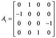 ,
, 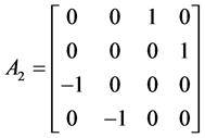 ,
,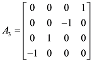 .
.
For N = 8 we have seven matrices with elements 0, ±1 [7] .
Let’s assume there is given a finite set of points of the function, called further nodes (xi, yi) Î R2 such as:
1) nodes (interpolation points) are settled at local extrema (maximum or minimum) and at least one point between two successive local extrema;
2) there are five nodes or more.
Assume that the nodes belong to a curve in the plane. How the whole curve could be reconstructed using this discrete set of nodes? Proposed method [8] [9] is based on local, orthogonal matrix operators. Values of nodes’ coordinates (xi, yi) are connected with HR matrices [10] build on N dimensional vector space. It is important that HR matrices are skew-symmetric and only for dimension N = 2, 4 or 8 columns and rows of HR matrices are orthogonal [1]">]">1] .
If one curve is described by a set of nodes  then HR matrices combined with identity matrix are used to build an orthogonal and discrete Hurwitz-Radon Operator (OHR). For nodes (x1, y1), (x2, y2) OHR of dimension N = 2 is constructed:
 . (2)
. (2)
For nodes (x1, y1), (x2, y2), (x3, y3), (x4, y4) OHR of dimension N = 4 is constructed:
 (3)
(3)
where
 ,
,  ,
,
 ,
, .
.
For nodes  OHR M of dimension N = 8 is built [8] similarly as Equation (3):
 (4)
(4)
where
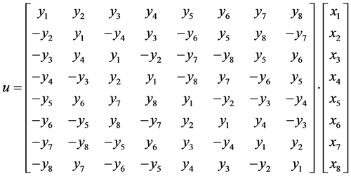 . (5)
. (5)
The components of the vector , appearing in the matrix M in Equation (4), are defined by Equation (5) in the similar way to Equations (2) and (3) but in terms of the coordinates of the above 8 nodes. Note that OHR operators in Equations (2)-(4) satisfy the condition of interpolation
 (6)
(6)
for , x ¹ 0,
  , N = 2, 4 or 8.
How can we compute coordinates of points settled between interpolation nodes? On a segment of a line every number “c” situated between “a” and “b” is described by a linear (convex) combination  for
for
 . (7)
. (7)
Average OHR operator M2 of dimension N = 2, 4 or 8 is constructed as follows:
 (8)
(8)
with the operator M0 built in Equations (2)-(4) by “odd” nodes  and M1 built in Equations (2)-(4) by “even” nodes
 . Notice that having the operator M2 for coordinates xi < xi+1 it is possible to reconstruct the second coordinates of points (x, y) in terms of the vector C defined with
 (9)
(9)
as . The required formula is adequate to Equation (6):
 (10)
(10)
in which components of vector Y(C) give us the second coordinate of the points (x, y) corresponding to the first coordinate, given in terms of components in Equation (9) of the vector C.
After computing in Equations (7)-(10) for any a Î [0;]">]">1], we have a half of reconstructed points (j = 1 in Algorithm 1). Now it is necessary to find second half of unknown coordinates (j = 2 in Algorithm 1) for
 (11)
(11)
There is no need to build the OHR for nodes  because we just find M1. This operator will play as role as M0 in Equation (8). New M1 must be computed for nodes
 . As we see the minimum number of interpolation nodes n = 2N + 1 = 5, 9 or 17 using OHR operators of dimension N = 2, 4 or 8 respectively. If there is more nodes than 2N + 1, the same calculations in Equations (7)-(11) have to be done for next range(s) or last range of 2N + 1 nodes. For example, if n = 9 then we can use OHR operators of dimension N = 4 or OHR operators of dimension N = 2 for two subsets of nodes:
  and
and . We summarize this section in the following algorithm of points reconstruction for 2N+1 = 5, 9 or 17 successive nodes.
Algorithm 1: let j = 1.
Input: Set of interpolation nodes {(xi, yi), i = 1, 2,×××, n; n = 5, 9 or 17}.
Step 1. Determine the dimension N of OHR operators: N = 2 if n = 5, N = 4 if n = 9, N = 8 if n = 17.
Step 2. Build M0 for nodes (x1 = a, y1), (x3, y3), ×××, (x2N−1, y2N−1) and M1 for nodes (x2 = b, y2), (x4, y4), ×××, (x2N, y2N) from Equations (2)-(4).
Step 3. Determine the number of points to be reconstructed Kj > 0 between two successive nodes, let k = 1.
Step 4. Compute a Î [0;]">]">1] from Equation (7) for c1 = c = a×a + (1 ‒ a)×b.
Step 5. Build M2 from Equation (8).
Step 6. Compute vector C = [c1, c2, ×××, cN]T from Equation (9).
Step 7. Compute unknown coordinates Y(C) from Equation (10).
Step 8. If k < Kj, set k = k + 1 and go to Step 4. Otherwise if j = 1, set M0 = M1, a = x2, b = x3, build new M1 for nodes (x3, y3), (x5, y5), ×××, (x2N+1, y2N+1), let j = 2 and go to Step 3. Otherwise, stop.
The number of reconstructed points in Algorithm 1 is K = N(K1 + K2). If there is more nodes than 2N + 1 = 5, 9 or 17, Algorithm 1 has to be done for next range(s) or last range of 2N + 1 nodes. Reconstruction of curve points using Algorithm 1 is called by author the method of Hurwitz-Radon Matrices (MHR).
3. MHR Calculations and Graphical Examples
In this section we consider the number of multiplications and divisions for MHR method during reconstruction of K = L ‒ n points having n interpolation nodes of the curve consists of L points. First we present a formula for computing one unknown coordinate of a single point. Assume there are given four nodes (x1, y1), (x2, y2), (x3, y3) and (x4, y4). OHR operators of dimension N = 2 are built in Equation (2) as follows:
 ,
, .
.
Let first coordinate c1 of reconstructed point is situated between x1 and x2:
 (12)
(12)
Compute second coordinate of reconstructed point y(c1) for Y(C) = [y(c1), y(c2)]T from Equation (10):
 (13)
(13)
After calculation by Equation (13):
 (14)
(14)
So each point of the curve P = (c1, y(c1)) settled between nodes (x1, y1) and (x2, y2) is parameterized by P(a) for Equations (12) and (14) and a Î [0;1].
If nodes (xi, yi) are equidistance in coordinate xi, then parameterization of unknown coordinate (14) is simpler. Let four successive nodes (x1, y1), (x2, y2), (x3, y3) and (x4, y4) are equidistance in coordinate xi and a = x1, h/2 = xi+1 ‒ xi = const. Calculations in Equations (13) and (14) are done for c1 in Equation (12):
 (15)
(15)
and
 . (16)
As we can see in Equations (15) and (16), MHR interpolation is not a linear interpolation. It is possible to estimate the in terpolation error of MHR method (Algorithm 1) for the class of linear function f:
 . (17)
Notice that estimation from Equation (17) has the biggest value 0.25çsç for b = a = 0.5, when c1 is situated in the middle between x1 and x2.
The goal of this paper is not a reconstruction of single point, like for example Equations (14) and (15), but interpolation of curve consists of L points. If we have n interpolation nodes, then there is K = L – n points to find using Algorithm 1 and MHR method. Now we consider the complexity of MHR calculations.
Lemma 1. Let n = 5, 9 or 17 is the number of interpolation nodes, let MHR method (Algorithm 1) is done for reconstruction of the curve consists of L points. Then MHR method is connected with the computational cost of rank O(L).
Proof. Using Algorithm 1 we have to reconstruct K = L – n points of unknown curve. Counting the number of multiplications and divisions D in Algorithm 1 here are the results:
D = 4L + 7 for n = 5 and L = 2i + 5;
D = 6L + 21 for n = 9 and L = 4i + 9;
D = 10L + 73 for n = 17 and L = 8i + 17;  □
□
The lowest computational cost appears in MHR method with five nodes and OHR operators of dimension N = 2. Therefore whole set of n nodes can be divided into subsets of five nodes. Then whole curve is to be reconstructed by Algorithm 1 with all subsets of five nodes: ,
,  ,
,  If the last node (xn, yn) is indexed n ≠ 4i + 1 then we have to use lastive nodes
  in Algorithm 1.
Function f(x) = 1/x is an example when the graph of interpolated function differs from the shape of polynomials considerably. Then classical interpolation is very hard because of existing local extrema of polynomial (Figure 1). Here is the application of Algorithm 1 for this function and five nodes.
Figure 2 contains not many interpolated points (twenty six) and minimal number of nodes (five), so numerical calculations of integral (precise value I = 2.196) by trapezoidal rule I1 = 2.213 are not always satisfying. Greater number of nodes and interpolated points gives us more accurate value of quadrature.
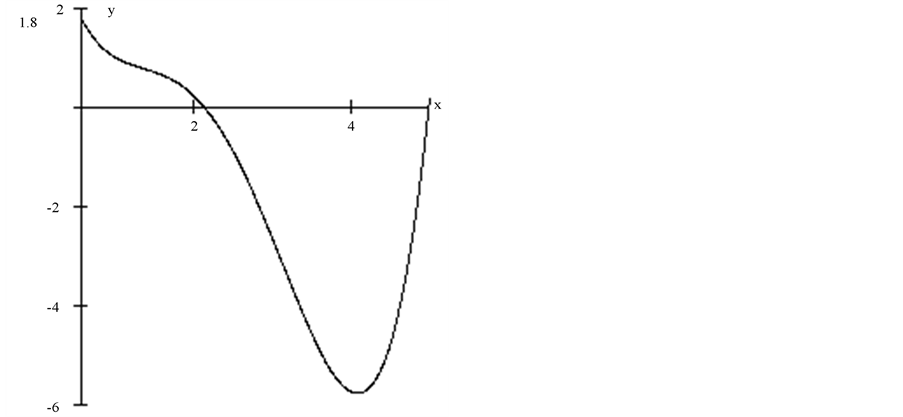
Figure 1. Lagrange interpolation polynomial of function f = 1/x differs extremely from the original.
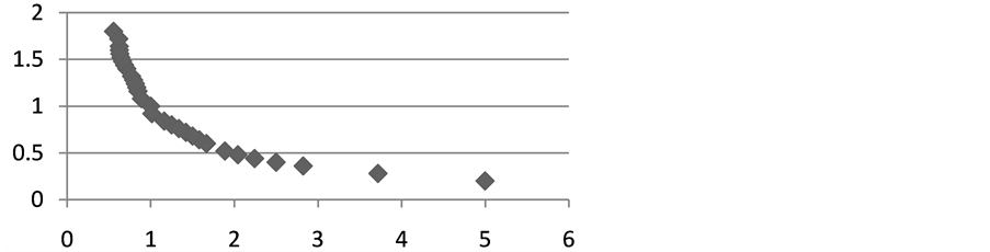
Figure 2.Twenty six interpolated points of function f = 1/x.
Lagrange interpolation polynomial for function f(x) = 1/x and nodes (5;0.2), (5/3;0.6), (1;1), (5/7;1.4), (5/9;1.8) has one local minimum and two roots.
Other examples of MHR interpolation and numerical quadratures:
Figure 3 contains minimal number of nodes (five) and not many interpolated points (twenty two), so numerical calculations of integral (precise value I = 0.549) are not always satisfying:
1) trapezoid method: I1 = 0.534;
2) Simpson’s rule: I2 = 0.538.
Greater number of nodes and interpolated points gives us more accurate value of quadrature.
Figure 4 contains minimal number of nodes (five) and not many interpolated points (thirty six), but numerical calculations of integral (precise value I = 1.029) are interesting:
1) trapezoid method: I1 = 1.000;
2) Simpson’s rule: I2 = 0.999.
After computing of K points for interpolated function (algorithm 1), it is possible to calculate the integral by trapezoid method or Simpson’s rule in range of each pair of successive interpolated points. Greater number of nodes and interpolated points gives us more accurate value of quadrature.
Figures 5-8 are the examples of interpolation for such functions as polynomial, logarithmic and exponential.
4. Summary
The method of Hurwitz-Radon Matrices (MHR-Algorithm 1) leads to curve interpolation depending on the number of nodes and location of nodes. No characteristic features of curve are important in MHR method: failing to be differentiable at any point, the Runge’s phenomenon or differences from the shape of polynomials.
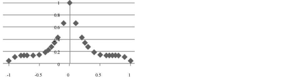
Figure 3. Function f = 1/(1 + 25x2), interpolated via MHR, without Runge phenomenon.
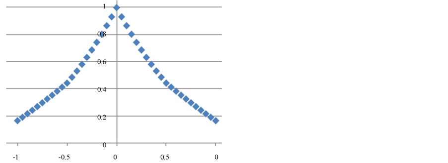
Figure 4. Function f = 1/(1 + 5x2), interpolated via MHR, without Runge phenomenon.
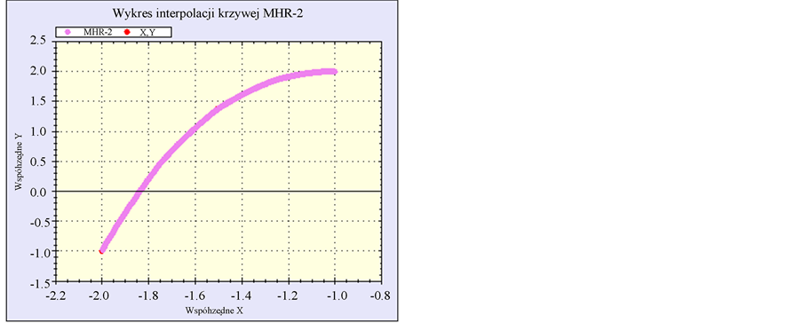
Figure 5. Function f(x) = x3 + x2 − x + 1 with 396 interpolated points using MHR method with 5 nodes: (−2; −1), (−1.75; 0.453125), (−1.5; 1.375), (−1.25; 1.859375) and (−1; 2).
These features are very significant for classical polynomial interpolations. MHR method gives the possibility of curve reconstruction and then numerical calculations of integrals for interpolated function via trapezoid method or Simpson’s rule for example. The only condition is to have a set of nodes according to assumptions in Algorithm 1. Curve modeling [12] by MHR method is connected with possibility of changing the nodes coordinates
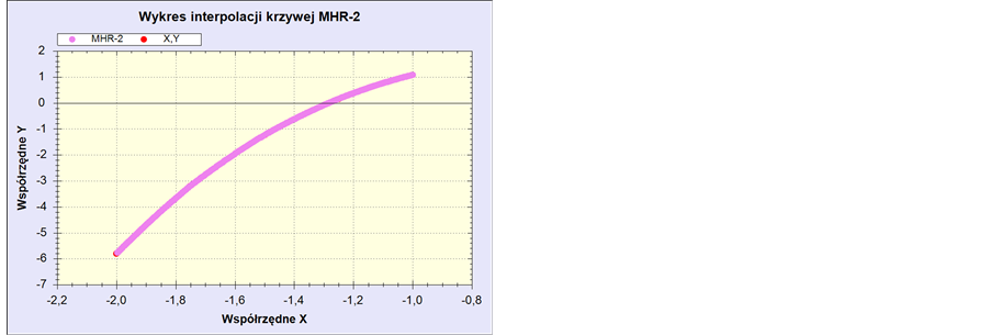
Figure 6. Function f(x) = x3 + ln(7 − x) with 396 interpolated points using MHR method with 5 nodes: (−2; −5.803), (−1.75; −3.190), (−1.5; −1.235), (−1.25; 0.1571) and (−1; 1.0794).
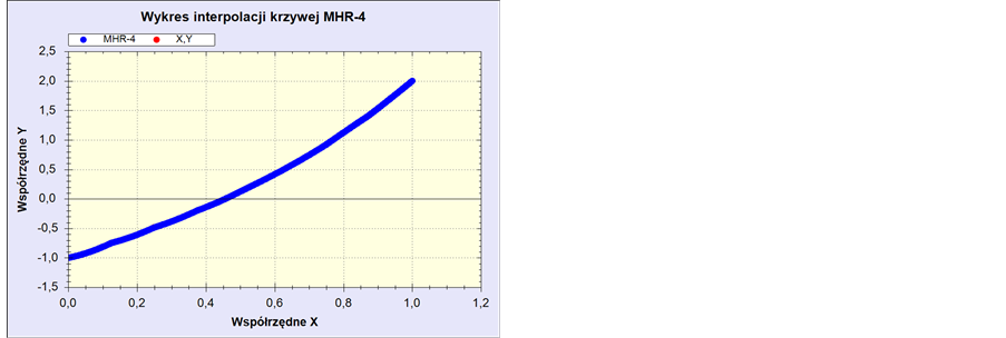
Figure 7. Function f(x) = x3 + 2x − 1 with interpolated points using MHR method with 9 nodes for xi = 0; 0.125; 0.25; 0.375; 0.5; 0.625; 0.75; 0.875 and 1.
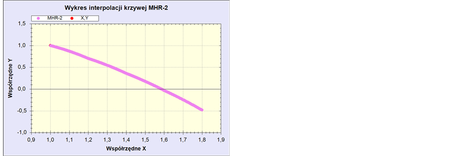
Figure 8. Function f(x) = 3 − 2x with 396 interpolated points using MHR method with 5 nodes: (1; 1), (1.2; 0.7026), (1.4; 0.361), (1.6; −0.031) and (1.8; −0.482).
and reconstruction of new curve or contour for new set of nodes, no matter what shape of curve or contour is to be reconstructed. Main features of MHR method are:
1) accuracy of curve reconstruction depending on number of nodes and method of choosing nodes;
2) Reconstruction of curve consisting of L points is connected with the computational cost of rank O(L);
3) Algorithm 1 is dealing with local operators: average OHR operator M2 (8) is built by successive 4, 8 or 16 nodes, what is connected with smaller computational costs then uses all nodes.
Future works are connected with: geometrical transformations of curve (translations, rotations, scaling)— only nodes are transformed and new curve (for example contour of the object) for new nodes is reconstructed; estimation of curve length [13] ; possibility to apply MHR method to three-dimensional curves [8] [9] ; object recognition [14] , shape representation [15] [16] and parameterization [17] in image processing; curve extrapolation [18] .
References
- Dahlquist, G. and Bjoerck, A. (1974) Numerical Methods. Englewood Cliffs N. J., Prentice-Hall.
- Jankowska, J. and Jankowski, M. (1981) Survey of Numerical Methods and Algorithms (Part I). Wydawnictwa Naukowo-Techniczne, Warsaw. (in Polish)
- Ralston, A. (1965) A First Course in Numerical Analysis. McGraw-Hill Book Company, Boston.
- Kozera, R. (2004) Curve Modeling via Interpolation Based on Multidimensional Reduced Data. Silesian University of Technology Press, Gliwice.
- Jakóbczak, D. (2009) Curve Interpolation Using Hurwitz-Radon Matrices. Polish Journal of Environmental Studies, 3B, 126-130.
- Citko, W., Jakóbczak, D. and Sieńko, W. (2005) On Hurwitz-Radon Matrices Based Signal Processing. Signal Processing’2005, Poznań, 19-24.
- Sieńko, W., Citko, W. and Jakóbczak, D. (2004) Learning and System Modeling via Hamiltonian Neural Networks. Lecture Notes on Artificial Intelligence, 3070, 266-271.
- Jakóbczak, D. (2007) 2D and 3D Image Modeling Using Hurwitz-Radon Matrices. Polish Journal of Environmental Studies, 16, 104-107.
- Jakóbczak, D. and Kosiński, W. (2007) Hurwitz-Radon Operator in Monochromatic Medical Image Reconstruction. Journal of Medical Informatics & Technologies, 11, 69-78.
- Eckmann, B. (1999) Topology, Algebra, Analysis—Relations and Missing Links. Notices of AMS, 46, 520-527.
- Lang, S. (1970) Algebra. Addison-Wesley Publishing Company, Boston.
- Jakóbczak, D. (2010) Object Modeling Using Method of Hurwitz-Radon Matrices of Rank k. In: Wolski, W. and Borawski, M., Eds., Computer Graphics: Selected Issues, University of Szczecin Press, Szczecin, 79-90.
- Jakóbczak, D. (2010) Shape Representation and Shape Coefficients via Method of Hurwitz-Radon Matrices. Lecture Notes in Computer Science, 6374, 411-419.
- Jakóbczak, D. (2011) Object Recognition via Contour Points Reconstruction Using Hurwitz-Radon Matrices. In: Józefczyk, J. and Orski, D., eds., Knowledge-Based Intelligent System Advancements: Systemic and Cybernetic Approaches, IGI Global, Hershey, 87-107.
- Jakóbczak, D. (2010) Application of Hurwitz-Radon Matrices in Shape Representation. In: Banaszak, Z. and swic, A. Eds., Applied Computer Science: Modelling of Production Processes, 1, Lublin University of Technology Press, Lublin, 63-74.
- Jakóbczak, D. (2010) Implementation of Hurwitz-Radon Matrices in Shape Representation. In: Choras, R.S., Ed., Advances in Intelligent and Soft Computing 84, Image Processing and Communications: Challenges 2, Springer-Verlag, Berlin Heidelberg, 39-50.
- Jakóbczak, D. (2011) Curve Parameterization and Curvature via Method of Hurwitz-Radon Matrices. Image Processing & Communications—An International Journal, 1-2, 49-56.
- Jakóbczak, D. (2011) Data Extrapolation and Decision Making via Method of Hurwitz-Radon Matrices. Lecture Notes in Computer Science/LNAI, 6922, 173-182.