ABSTRACT

We start where we use an inflaton value due to use of a scale factor $a~a_{\min }{t}^{\gamma }$ . Also we use $\delta g_{tt}~a_{\min }^2\cdot {\varphi }_{\text{initial}}$ as the variation of the time component of the metric tensor $g_{tt}$ in Pre-Planckian space-time. Our objective is to find an effective magnetic field, to obtain the minimum scale factor in line with Non Linear Electrodynamics as given by Camara, et al., 2004. Our suggestion is based upon a new procedure for an effective current based upon an inflaton time exp (i times (frequency) times (cosmological time)) factor as a new rescaled inflaton which is then placed right into a Noether Current scalar field expression as given by Peskins, 1995. This is before the Causal surface with which is, right next to a quantum bounce, determined by $H_{\text{causal-structure-quantum-bounce}}=0$ , with the next shift in the Hubble parameter as set up to be then $H_{\text{initial}}~1/\Delta t~1.66\sqrt{g_{*}}\cdot T^2/M_{\text{mass-scale}}$ . And $g_{*}$ is an initial degree of freedom value of about 110. Upon calculation of the current, and a resulting magnetic field, for the space time bubble, we then next obtain a shift in energy, leading to a transition from $H_{\text{causal-structure-quantum-bounce}}=0$ too. We argue then that the delineation of the $\delta g_{tt}~a_{\min }^2\cdot {\varphi }_{\text{initial}}$ term is a precursor to filling in information as to the Weyl Tensor for near singularity measurements of starting space-time. Furthermore, as evidenced in Equations ((26) and (27)) of this document, we focus upon a “first order” that checks into if a cosmological “constant” would be invariant in time, or would be along the trajectory of the time, varying Quinessence models. We close this document, with Maxwell equations as to Post Newtonian theory, for Gravity, with our candidates as to a magnetic field included in, with what we think this pertains to, as far as Gravo Electric and Gravo Magnetic fields, and then make suggestions as to a quantum version of this methodology for future gravitational wave physics research. This is Appendix G, this last topic, and deliberately set up future works paradigm which will be investigated in the coming year. It is based upon a Gravo Electric potential, and we make suggestions as to its upgrade in our future works, in early universe cosmology. In the reference by Poisson, and Will, they write ${\left(v/c\right)}^2=1-4U/c^2$ and in this last section we come up with a value of U, based in part on the comparison with the alteration of velocity, due to a massive graviton, namely via the substitution, we write as ${\left(v/c\right)}^2=1-4U/c^2=1-\frac{m_g^2{c}^4}{E_{\text{Graviton}}^2}$ , so as to come up with a post Newtonian approximation result for a magnetic field. We compare this magnetic field, as far as the Inflaton magnetic field, and use it to come up with observations with regards to the phenomenology of gravity in Pre Planckian to Planckian regime limits. We close, then with the observation given in Appendix H, of the inhomogeneity of Pre Planckian-to Planckian space time as a necessary condition for a Gravi-Magnetic field. We also reference an Appendix I, which does a summary of a 5^th force calculation, and we then compare those results, with our temporary results of a Gravi Magneitc field, as we have tried to start up as a future works project.

Keywords:

Inflaton Physics, Causal Structure, Penrose Weyl Tensor Conjecture, Quinessence, Gravo Electric Potential Gravo Electric and Gravo Magnetic Fields

1. Outlining an Inflaton Model, Which Is Pertinent, to the Physics Just in the Vicinity of a Quantum Bounce

We wish to state that our paper is an extension of the initial manuscript, as given by the author, in [1] and is to answer a question which has vexed the author repeatedly. If magnetic fields exist at the start of the universe, then what creates them?

Our solution is to base a current, for the magnetic field, as created by a Noether current [2] , as a starting point, with the Noether current created as partly derived from an inflaton field, times exponential of the imaginary number, frequency, and time interval. In doing so, our derived Noether current is real valued, which is astonishing, and is part of the reason we call this effective current as the actual current of an initial relic gravitational field.

We will now commence introducing the scalar field, we will use repeatedly.

We will begin using the physics outlined in [3] as to

(1)

Our starting point in this Linde result [3] , is to utilize the Beckwith-Moskaliuk, vresult that [4]

(2)

Utilizing here that, [4] [5]

(3)

If so then we have, approximately a use of, by results of Sarkar, as in [6]

(4)

in terms of early universe Hubble expansion behavior which we incorporate into our uncertainty principle, to obtain

(5)

And by Padmanabhan [7] for the interior of the bubble of space-time, we will have, here that

(6)

From here, we will explain the behavior of a change in energy about the structure of a Causal boundary of the bounce bubble in space-time defined by Beckwith, in [1] so that

(7)

Here, in doing so, to fill in the details of Equation (4), we will be examining the Camara et al. result of [8]

$\begin{array}{l}{a}_{\min }~{\alpha }_0\cdot {\left(\frac{{\alpha }_0}{2\tilde{\lambda }}\cdot \left(\sqrt{{\alpha }_0{}^2+32\text{π}{\mu }_0\omega \cdot B_0^2}-{\alpha }_0\right)\right)}^{1/4}\\ {\alpha }_0=\sqrt{\frac{4\text{π}G}{3{\mu }_0{c}^2}}{B}_0\\ \tilde{\lambda }=\frac{{\Lambda }_{\text{Einstein}}{c}^2}{3}\end{array}$ (8)

Specifically, we will be filling in the details of Equations ((1) to (8)) with the adage that we will be using of all things, a modified version of the Noether Current, [2] according to a simplified version of the treatment given in [8] with a scalar field, we will define as

(9)

which will allow, after calculation, that the Noether current will be, if linked to its time component, real valued, which is a stunning result. Our next trick will be then to put this effective quantum bubble “current” as the magnetic field, B₀, using the results of both Gifffiths, [9] and Landau and Liftschitz, [10] for a magnetic field, for Equation (7). This, then will be the plan of what we will be working with in this article, in subsequent details.

2. Making a Statement about a Constituent Early Universe Magnetic Field

We start off with Ohm’s law [9] [10] [11] assuming a constant velocity within the space-time bubble, of

(10)

Where the velocity of some “particle”. Or energy packet, or what we might call it, does not change. Then use the Griffith’s relationship [9] of

(11)

We will comment upon the σ later, but first say something about what j as current is proportional to the modus operandi chosen here is to employ the following. Use a scalar field defined by Equation (9) and a Noether conserved current [3] proportional to:

(12)

Here we take the time component of this Noether current, and use Equation (9) for $\tilde{\varphi }$ , and Equation (6) for f. Therefore

(13)

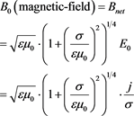
Then our net magnetic field, is to first approximation given by

(14)

This is to be put into our value of Equation (8) above. So, next we will be looking at the frequency, ω.

3. Rule of Thumb Estimates for Frequency, ω

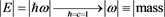
We will go on the meme of an admissible low to high value for the imput frequency. First of all the high frequency limit. This comes from an argument from Ford [12] i.e. for a black hole of mass M to evaporate, we have

(15)

If we make the assumption, that a white hole, is an evaporating black hole, i.e. and then up the mass, M, from a solar sized black hole, to a white hole, as the starting point for cosmological evolution, according to [13] as given by Mueller, and Lousto, we have that for a small radii less than one Plank length diameter starring point for a black hole, with the approximation given dimensionally, that

(16)

Then, this means, that the upper limit of frequency, in this case could be effectively infinite, Now that we have an argument in place for an upper limit, what about the lower limit? To do this, assume the following i.e. assume a Planck radii for the bubble of space-time. i.e. up to a point this would signify a frequency range of say 10³⁵ Hertz, initially, and then for today, consider that if there are 65 e folds of inflation, that Frequency range is, then for the lower bound given by

(17)

i.e. this means that the initial frequency is initially nearly infinite, to at lowest 10³⁵ Hertz (initial) With that, we can also take a look at an estimate as to conductivity, which is given by Ahonen and Enqvist [14] to be about σ ≃ 0.76T while at T ≃ M_W [14] will obtain σ ≃ 6.7 T, and we can tie that as similar to the strength of the magnetic fields given in [15] as well.

Note that the electrical conductivity is used here, with the conversion between an E field to a B field, in magnitude given by Equation (11)

In all, with all the assumptions so used, we have that [8]

(18)

4. Parameterizing the Role of Equation (4) in Our Model, and Its Importance.

What we have done, is to set up the way which we can obtain inputs into

$\Delta E~\frac{{\left(1.66\cdot \sqrt{g^{\ast }}\cdot \frac{T_{\text{Early-Universe}}}{M_{\text{mass-scale}}}\right)}^3\cdot \hslash }{{\left(2\text{π}{a}_{\min }\right)}^2{\varphi }^3}$

$\begin{array}{l}~\frac{{\left(1.66\cdot \sqrt{g^{\ast }~110}\cdot \frac{T_{\text{Early-Universe}}}{\left(M_{\text{mass-scale}}\approx {10}^{43}\cdot M_{\text{Planck}}\right)}\right)}^3\cdot \hslash }{{\left(2\text{π}\cdot {10}^{-55}\right)}^2\cdot {\left(\sqrt{\frac{\gamma }{4\text{π}G}}\cdot \left[\sqrt{\frac{8\text{π}G\cdot V_0}{\gamma \cdot \left(3\gamma -1\right)}}\cdot \Delta t-1\right]/\sqrt{\frac{8\text{π}G\cdot V_0}{\gamma \cdot \left(3\gamma -1\right)}}\cdot \Delta t\right)}^3}\\ \propto M_{\text{mass-scale}}\approx {10}^{43}\cdot M_{\text{Planck}}\end{array}$ (19)

Doing it this way, i.e. having the change in energy, crossing the causal boundary of specified Equation (8) puts a very strong set of constraints upon the allowed values of V₀, σ. γ, and Dt on top of and

What is being said, is that the above Equation (19) puts in a range of admissible values on V₀, σ. γ, and Dt on top of and in addition to the frequency, which is referenced in section 3 of this manuscript. In doing so the idea is to come up with experimental constraints which will validate a range of experimental gravitational inputs into evaluation of presumed early universe data sets.

This should be compared to an earlier relationship given by Beckwith at [1] which has, if

(20)

We claim that all three of these Equation (18) to Equation (20) are inter related. And are part of potential data analysis in our problem.

It also depends, upon, critically, that k (curvature), for initial curvature be finite and nonzero.

5. Revisiting What Can Be Said about the Weyl Tensor

We initiate this section by stating the n = 4 (three spatial dimensions and one time dimension) Weyl Tensor, in the case of a Friedman-Lemaitre-Roberson-Walker metric given by [1] [16] which we rewrite as

(21)

The entries into the above, assuming c = 1 (speed of light) in the Friedman-Lemaitre-Roberson-Metric would be right after the Causal boundary given as [1] [17] , namely if we go by [18]

(22)

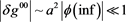
In our rendering of what to expect, we will be setting k (curvature), initially as not equal to zero, and that the minimum value of the scale factor, be defined by. If so then

(23)

If so, then approximate having

(24)

And, up to first order, replace one item by

$\begin{array}{c}{g}_{00}=-1+\delta g_{00}\\ =-1+a_{\text{initial}}^2\cdot \sqrt{\frac{\gamma }{4\text{π}G}}\cdot \left(\left[\sqrt{\frac{8\text{π}G\cdot V_0}{\gamma \cdot \left(3\gamma -1\right)}}\cdot \Delta t-1\right]/\sqrt{\frac{8\text{π}G\cdot V_0}{\gamma \cdot \left(3\gamma -1\right)}}\cdot \Delta t\right)\end{array}$ (25)

With the rest of the items in Equation (22) for the metric tensor held the same. i.e. then we would have, if r in Equation (22) were of the order of Planck length, that the Weyl tensor, would not necessarily vanish, no matter how close one got to the purported singularity.

We refer the readers to Appendix A, which highlights the inter relationship of the Weyl Tensor to some of the other tensors of General relativity.

The details of this are being reviewed, with a Phase transition model for the transition to Pre Planckian to Planckian physics still in the works.

We submit that one of the goals of our paper would be to construct, a template which would justify the existenc3e of massive Gravitons, and we allude to this in Appendix B, which incidently mentions the inter connections of the Weyl Tensor, and (E, B) fields with (j = current, ρ = density) explicitly.

6. Conclusions

Much to do, i.e. the details are daunting and depend upon confirmation of the idea of the current in Pre Planckian to Planckian space time proportional to a Noether current, being confirmed and verified.

The main crust of our approach is to come up with a thought experiment as to the creation of a Noether style based current, as would be enabler of a magnetic field, at the start of Planckian space-time dynamics.

Note that in Appendix C, we review what can be said about the semi classical nature, versus quantum generation of, and if or not our results are linked to new properties, of Gravitational waves. In fact, we do believe this is the case, and before we get to that, we will review some stated issues as to initial curvature, i.e. much of what we are doing is linked to an early Universe version of a small, but non vanishing curvature value, which depends in part on some of the issues brought up in Appendix C.

In addition, Appendix D, says something about what may be expected, in terms of new features to be considered as far as GW and LIGO style instruments.

Our informed guess is that we will in the end write the initial curvature along the lines of it having the form

(26)

i.e. this would be very small, but not zero. The fact it was small, but not zero, even in the Pre Planckian regime of space-time would be of supreme importance, and would affect the evolution of subsequent space-time.

Linking this result, above, to confirmation of the above Equation (20) would tend to, aside from root finder methods outlined by the author, lend itself to a bounding value of a discrete time step, we will write as

(27)

i.e. to solve for Dt would involve a transcendental non linear root finder scheme, but this could be matched against an earlier result which was represented in [1] as

(28)

Doing so, and making equivalence, if we use Equation (27) to solve for Dt and use Equation (28) to parameterize the Cosmological “constant” in our early universe cosmology, would be among other things a way to address the issue of Quinessence, i.e. would the cosmological constant evolve in time, or would the results of Equation (28) after using Equation (27) for confirming a value of Dt give credence to the idea of the invariance of the cosmological constant?

This we view as a worthy investigative topic, and one within our reach.

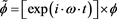
Aside from that, the idea of using a Noether current based upon the idea of a scalar field which is based upon inflaton time exp (i times frequency times time) factor would give a foundational treatment of Non linear electrodynamics magnetic fields as has been brought up by several authors, the writer of this manuscript counts as peers and worthy researchers.

Prior treatments of the scalar fields used in Noether’s theorem talk of having a tie in with early universe magnetic fields.

What is being done in this manuscript, is to purport, that the idea should be to make the derived Noether’s current the core of a magnetic field, and from there to also do it along the ideas brought up in the manuscript, in a reversal of the usual order of tying in the scalar field, directly with early universe magnetic fields.

The exponential factor of, which is multiplied into an inflaton field, makes the Noether current we derive real valued. This will allow us more background in investigating what Corda brought up in [19] .

Moreover, in doing so, we are giving a foundational derivation of a magnetic field which is used by, Camara [8] , and other researchers in Non Linear electrodynamics, as to cosmology, which is a necessary appendage as to the inflaton based creation of a magnetic field, at the start of cosmological evolution.

In doing all of this, Corda’s suggestions as to how early universe conditions can be used to investigate the origins of gravity [19] take on a new significance.

We also, by tying in our work so closely to the origins of a new magnetic field, which we also state will be important to relic graviton production, give new urgency to necessary reviews of Abbot, and the LIGO team as to the evolving experimental science of gravitational astronomy. [20] [21] .

To see what we are referring, to go to Appendix C, and note what we are referencing are necessary conditions on if, or not early universe GW have semi classical, or mainly quantum mechanical initial conditions.

Finally, our suggestions as to a start to the Weyl Tensor problem need to be confirmed and held to be in congruence, with the positions given above.

Note this is in connection to the interior boundary of space-time. And that our supposition will be matched to a causal boundary barrier between the initial boundary of a quantum bubble, and Huang’s super fluid universe, post causal boundary barrier, which we write as [1] [18]

$H^2=\frac{-k\left(\text{curvature}\right)}{a^2}+\frac{2}{3}\cdot {\rho }_c$

$\begin{array}{l}\&{\rho }_c=\frac{{\dot{\varphi }}^2}{2}+V\left(\varphi \right)\\ \&H^2\left(\text{Quantum-bounce}\right)=0\\ \iff a^2=\frac{3k\left(\text{curvature}\right)}{2{\rho }_c}\\ \iff a_{\text{bounce}}=\sqrt{\frac{3k\left(\text{curvature}\right)}{{\dot{\varphi }}^2+2V\left(\varphi \right)}}\end{array}$ (29)

It finally would be a way to investigate some issues raised in [22] , as well as the idea, generically of a Gyraton, [1] [23] [24] which may be a candidate for a Pre-inflaton graviton.

Our future projects, will be along the lines of what is mentioned in [25] , as far as higher dimensional versions of the Weyl tensor. The idea will be if we do not have initial singularities mandated at the start of cosmological evolution to revisit some of the ideas held up as the gold standard in [26] , as well as to also investigate the role of five dimensional cosmologies brought up by Wesson in [27] . In doing so, we recommend that the readers look at exact solutions of the Einstein equations brought up in [28] before commencing their own projects due to how hard the ideas of this inquiry really are.

Note in Appendix D, we also will bring up one of the hoariest predictions as far as Signal to noise ratios, in gravitational wave astronomy. i.e. we will briefly bring up the LIGO results, as far as Signal to noise, and to then postulate a different set of rules as far as what to expect in Signal to noise, as far as relic Gravitational wave production due to Graviton production in the early universe.

If we review the results of Appendix D, and find they tend to a production for gravitons at the surface of a causal bubble, it will be then time to go to Appendix E, whereas we discuss the frankly startling phenomenological considerations as to the phase factor of times a derived Noethers current with the scalar field, as used, for the Noethers current being the inflaton itself.

As asked in questions to the author by a referee,

Quote

“The exponential factor of exp(i w t), which is multiplied into an inflation field, makes the Noether current we derive real valued. This will allow us more background in investigating what Corda brought up in [19] .” So, the most important question is: what is the reason to use exp(i w t) element to compare with your new results and I think it needs to be described in details to cover the results in [19] [20] [21] ?

End of quote

In partial answer, this is linked to earlier work which the author presented in a generalization of cyclic conformal cosmology, to a multiverse setting, for reasons which will be gone into, in Appendix E

We will tend toward the result that in the center of a cosmological bubble of space-time, that we set will tend to be 1, whereas, at the boundary of the bubble, that we, again have that the will tend to be 1, with the result that, among other things, we will have the following relationship between frequency, and an initial time step, i.e. at the boundary of space time, with the frequency, so configured, having a minimum value of

If we configure this as linkable to input into the relic early universe gravity waves/gravitons, and compare it against what we are predicting as far as signal to noise ratios, this says something potentially quite profound as far as relic Gravitational waves, based upon a graviton model. Something which may be definable, and a falsifiable experimental datum in Gravitational wave astronomy.

We leave Appendix F for a subsequent round up and summarizing of the main significant points of our document, as well as further answers to the issues brought up by the Referee, which may have significant phenomenological import, in terms of turning Gravitational wave astronomy into a rigorous falsifiable scientific discipline enabling us to explore cosmology on an empirical basis.

In lieu of the nonstandard situation of this paper, Appendix F has the referees comments, and my detailed replies.

We close the physics ideas of the main text with Appendix G, which first of all recapitulates points made in a book, by Poissons, and Clifford Will, as to Maxwell like Formulation of Post Newtonian Theory, in which we add in, instead of what was given in the book for Maxwell equations as to Post Newtonian theory, for Gravity, our candidates as to a magnetic field included in, with what we think this pertains to, as far as Gravo Electric and Gravo Magnetic fields, with a suggestion as to the phenomenological import of this to Gravity waves.

Appendix H, as given makes a reference as to Gravo Magnetic fields being modified, by the import of deformation mechanics, i.e. how we can approach the commutation values of Quantum mechanics.

And then finally we then use Appendix I to briefly allude to the ideas of Fifth forces, as we present a problem, i.e. we have a different current calculation as to the Magnetic field.

This last section can be reformulated in the future and possibly improved to come up with some new physics as to early Universe Gravitational Waves, but we should in passing make reference to the following, as quoted in Appendix I, the following should be kept in mind.

Quote (From Appendix I)

So, what is the upshot? We can say clearly, that the magnetic field, so obtained, does not look ANYTHING like our value of magnetic field. Why? Simply put, we are using a very different CURRENT. i.e. our current used in the main part of the text, is dependent upon an INFLATON, and that even in Appendix G, and Appendix H, where we take care to use Maxwell’s Equations, we have a very different genesis of a magnetic field. i.e. Equation (I 19) has no similarities to Equation (14) of the main text.

i.e. our Fifth force calculation is dependent upon charges, and there is a very real question of if we have charges, formed, in the Pre Planckian to Planckian regime of space-time.

i.e. possibly as brought up by Steinhardt, in private conversations, we could recycle gravitons and maybe other such material from a prior universe, to the present universe, but this is highly suppositional.

The main difference between our main text result, and the fifth force approach outlined here is in the origins of the presumed current. And this needs to be somehow resolved, via experimental data sets.

End of Quote

Our open final question;. Is it meaningful to refer to magnetic fields in the genesis of the early universe in terms of charges? i.e. without the current we derived?

Appendix I shows a fifth force calculation for the magnetic field, and if we do it, still using ‘traditional charges’ we come up with a vastly different B field. i.e. the B field of Appendix I, and what we have in Appendix G, and Equation (14) are vastly different.

Setting the origins of a presumed current, in Pre Planckian to Planckian physics, is extremely important for understanding the fidelity of our experimental data sets to models we pick for the origins of space ? time evolution.

Acknowledgements

This work is supported in part by National Nature Science Foundation of China grant No. 1137527.

Cite this paper

Beckwith, A.W. (2018) How to Determine a Jump in Energy Prior to a Causal Barrier, with an Attendant Current, for an Effective Initial Magnetic Field. In the Pre Planckian to Planckian Space-Time. Journal of High Energy Physics, Gravitation and Cosmology, 4, 323-353. https://doi.org/10.4236/jhepgc.2018.42021

References

Appendix A: What Can Be Said about the Weyl Tensor in Connection to the Other Tensors of General Relativity

The formulas are based on [29] whereas an additional commentary is included from [30]

We start off with a description of the inter relationship of the different Tensors of General relativity, noting that [29] gives us that for n (dimensions) greater than or equal to 3, that the Curvature Tensor is written as

$\begin{array}{c}{R}_{\lambda \mu \nu \kappa }=\frac{1}{\left(\stackrel{⌣}{n}-2\right)}\cdot \left(g_{\mu \nu }{R}_{\mu \kappa }-g_{\lambda \kappa }{R}_{\mu \nu }-g_{\mu \nu }{R}_{\lambda \kappa }+g_{\mu \kappa }{R}_{\lambda \nu }\right)\\ +\frac{R}{\left(\stackrel{⌣}{n}-1\right)\left(\stackrel{⌣}{n}-2\right)}\cdot \left(g_{\lambda \nu }{g}_{\mu \kappa }-g_{\lambda \kappa }{g}_{\mu \nu }\right)+C_{\lambda \mu \nu \kappa }\end{array}$ (A1)

Here, $C_{\lambda \mu \nu \kappa }$ is the Weyl tensor, $R_{\lambda \mu \nu \kappa }$ is the curvature tensor, and R is the curvature scalar defined by [29]

$R=\frac{R_{1212}}{g}=\frac{R_{1212}}{\det \left(g_{\mu \nu }\right)}$ (A2)

$g_{\mu \nu }$ represents components of the Metric Tensor, and $\stackrel{⌣}{n}$ is the dimension of space-time assumed. Here,

$\begin{array}{c}{R}_{\mu \kappa }=g^{\lambda v}{R}_{\lambda \mu \nu \kappa }=\frac{g^{\lambda v}}{2}\cdot \left[\frac{{\partial }^2{g}_{\nu \lambda }}{\partial x^{\kappa }\partial x^{\mu }}-\frac{{\partial }^2{g}_{\mu \nu }}{\partial x{}^{\kappa }\partial x^{\lambda }}-\frac{{\partial }^2{g}_{{}^{\lambda \kappa }}}{\partial x^{\nu }\partial x^{\mu }}+\frac{{\partial }^2{g}_{\mu \kappa }}{\partial x^{\nu }\partial x^{\lambda }}\right]\\ +g^{\lambda v}{g}_{\eta \sigma }\cdot \left({\Gamma }_{\nu \lambda }^{\eta }{\Gamma }_{\mu \kappa }^{\sigma }-{\Gamma }_{\kappa \lambda }^{\eta }{\Gamma }_{\nu \eta }^{\sigma }\right)\end{array}$ (A3)

While the Affine connection ${\Gamma }_{\mu \kappa }^{\sigma }$ [31] , with $g^{im}$ the inverse matrix of $g_{im}$ , with a defining quantity of

${\Gamma }_{kl}^i=\frac{g^{im}}{2}\cdot \left[\frac{\partial g_{m,k}}{\partial x^l}-\frac{\partial g_{ml}}{\partial x{}^{\kappa }}+\frac{\partial g_{kl}}{\partial x^m}\right]$ (A4)

Note that Penrose in [30] defines the Weyl Tensor, as the Gravitational field analogy to the Maxwell Tensor, in terms of Electromagnetic E and B fields. As given on page 211 of his reference [30] . We say,more about this in Appendix B, next, and reference it as to massive gravitons.

Appendix B: Massive Gravitons, and the Weyl Tensor, and Electromagnetics

In reference [30] , Penrose writes the identification of the three tensors in pages 210-211 of [30]

RIEMANN (Curvature Tensor) = Weyl Tensor + Ricci Tensor (B1)

We have already made an identification of this in Equation (A1) of Appendix A. What Penrose has done next, is to make the following identification, namely on page 210 of [30]

Ricci Tensor = Energy (B2)

In doing so, what we will assert, is the following equivalence, near an almost singular configuration of space-time

Energy = RIEMANN (Curvature Tensor) − Weyl Tensor (B3)

Our supposition is that the Weyl Tensor does not vanish, but instead is a nonzero, but small component Note, that we have a massive graviton, as given by [32] , where we could easily have the massive Graviton as equivalent to roughly about 10⁻⁶² grams, i.e. and this by [33]

The relevant energy which we will be examining, will be through an adaptation of [30] and [33] and Equation (B3)

$\begin{array}{c}\text{Energy}~\frac{1}{\left(\stackrel{⌣}{n}-2\right)}\cdot \left(g_{\mu \nu }{R}_{\mu \kappa }-g_{\lambda \kappa }{R}_{\mu \nu }-g_{\mu \nu }{R}_{\lambda \kappa }+g_{\mu \kappa }{R}_{\lambda \nu }\right)\\ +\frac{R}{\left(\stackrel{⌣}{n}-1\right)\left(\stackrel{⌣}{n}-2\right)}\cdot \left(g_{\lambda \nu }{g}_{\mu \kappa }-g_{\lambda \kappa }{g}_{\mu \nu }\right)\end{array}$ (B4)

Note that in writing this up, we are assuming that the energy, in doing this has several equivalences which we write here, namely

In lieu of our derivation of the magnetic field, that one of the treatments of the available energy, in this case is by [34]

$\text{Energy}~\text{Volume}\cdot \frac{B^2}{8\text{π}}$ (B5)

However, we can only have a nonzero INITIAL volume, if the Weyl Tensor, as we define it is NOT equal to zero!

Hence, taking the square of the magnetic field, we will have

$\begin{array}{c}\text{Energy}~\text{Volume}\cdot \frac{1}{8\text{π}}\cdot {\left(\frac{\sqrt{\epsilon {\mu }_0}}{\sigma }\cdot {\left(1+{\left(\frac{\sigma }{\epsilon {\mu }_0}\right)}^2\right)}^{1/4}\cdot \frac{\gamma }{2\text{π}G}\cdot \frac{\omega }{\Delta t}\cdot \left[1-\frac{1}{\Delta t}\cdot \sqrt{\frac{\gamma \cdot \left(3\gamma -1\right)}{8\text{π}G\cdot V_0}}\right]\right)}^2\\ ~N\left(\text{graviton-number}\right)\cdot m_g\left(\text{graviton-mass}\right)\end{array}$ (B6)

i.e. we will be assuming here that $N\left(\text{graviton-number}\right)$ is a count of initial entropy, and that in lieu of a Weyl Tensor not vanishing at a non existent singularity, we have, say

$\text{Volume}~{\left(l_{\text{Planck}}\right)}^{\stackrel{⌣}{n}}$ (B7)

This will set up the following equivalence, namely

$\begin{array}{c}\text{Energy}~{\left(l_{\text{Planck}}\right)}^{\stackrel{⌣}{n}}\cdot \frac{1}{8\text{π}}\cdot (\frac{\sqrt{\epsilon {\mu }_0}}{\sigma }\cdot {\left(1+{\left(\frac{\sigma }{\epsilon {\mu }_0}\right)}^2\right)}^{1/4}\cdot \frac{\gamma }{2\text{π}G}\\ \cdot {\frac{\omega }{\Delta t}\cdot \left[1-\frac{1}{\Delta t}\cdot \sqrt{\frac{\gamma \cdot \left(3\gamma -1\right)}{8\text{π}G\cdot V_0}}\right])}^2\\ ~N\left(\text{graviton-number}\right)\cdot m_g\left(\text{graviton-mass}\right)\\ ~\frac{1}{\left(\stackrel{⌣}{n}-2\right)}\cdot \left(g_{\mu \nu }{R}_{\mu \kappa }-g_{\lambda \kappa }{R}_{\mu \nu }-g_{\mu \nu }{R}_{\lambda \kappa }+g_{\mu \kappa }{R}_{\lambda \nu }\right)\\ +\frac{R}{\left(\stackrel{⌣}{n}-1\right)\left(\stackrel{⌣}{n}-2\right)}\cdot \left(g_{\lambda \nu }{g}_{\mu \kappa }-g_{\lambda \kappa }{g}_{\mu \nu }\right)\end{array}$ (B8)

Appendix C. Are Relic Initially Generated Gravity Waves, Semi Classical, or Quantum in Origin? i.e. A Review of the NG Infinite Quantum Statistics Idea Entropy Generation via Ng’s Infinite Quantum Statistics (Short Review)

We wish to understand the linkage as. how relic gravitational waves relate to relic gravitons”?, To consider just that, we look at the “size” of the nucleation space, V for dark matter, DM. V for nucleation is HUGE. Graviton space V for nucleation is tiny, well inside inflation. Therefore, the log factor drops OUT of entropy S if V chosen properly for both Equations ((C1) and (C2)). Ng’s result [35] [36] begins with a modification of the entropy/partition function Ng used the following approximation of temperature and its variation with respect to a spatial parameter, starting with temperature $T\approx R_H^{-1}$ ( $R_H$ can be thought of as a representation of the region of space where we take statistics of the particles in question). Furthermore, assume that the volume of space to be analyzed is of the form $T\approx R_H^3$ and look at a preliminary numerical factor we shall call $N~{\left(R_H/l_P\right)}^2$ , where the denominator is Planck’s length (on the order of 10⁻³⁵ centimeters). We also specify a “wavelength” parameter $\lambda \approx T^{-1}$ . So the value of $\lambda \approx T^{-1}$ and of $R_H$ are approximately the same order of magnitude. Now this is how Jack Ng changes conventional statistics: he outlines how to get $S\approx N$ , which with additional arguments we refine to be $S\approx \langle n\rangle$ (where $\langle n\rangle$ is graviton density). Begin with a partition function

$Z_N~\left(\frac{1}{N!}\right)\cdot {\left(\frac{V}{{\lambda }^3}\right)}^N$ (C1)

This, according to Ng, leads to entropy of the limiting value of, if $S=\left(\log \left[Z_N\right]\right)$

$S\approx N\cdot \left(\log \left[V/N{\lambda }^3\right]+5/2\right)\underset{\text{Ng-infinite-Quantum-Statistic}}{\to }N\cdot \left(\log \left[V/{\lambda }^3\right]+5/2\right)\approx N$ (C2)

But $V\approx R_H^3\approx {\lambda }^3$ , so unless N in Equation (C2) above is about 1, S (entropy) would be < 0, which is a contradiction. Now this is where Jack Ng introduces removing the N! term in Equation (C1) above, i.e., inside the Log expression we remove the expression of N in Equation (0.2) above. The modification of Ng’s entropy expression is in the region of space time for which the general temperature dependent entropy Kolb and Turner expression breaks down. In particular, the evaluation of entropy we do via the modified Ng argument above is in regions of space time where g before re heat is an unknown, unmeasurable number of degrees of freedom The Kolb and Turner entropy expression [37] (1991) has a temperature T related entropy density which leads to that we are able to state total entropy as the entropy density time’s space time volume $V_4$ with $g_{\text{re-heat}}\approx 1000$ , while dropping to $g_{\text{electro-weakt}}\approx 100$ [37] in the electro weak era. This value of the space time degrees of freedom, has reached a low of $g_{\text{today}}\approx 2\text{-}3$ today. We assert that Equation (C2) above occurs in a region of space time before $g_{\text{re-heat}}\approx 1000$ , so after re heating Equation (2) no longer holds, and we instead can look at [37]

(C3)

where $T<{10}^{32}\text{K}$

Note that the result, as to Gravity waves, if given by the entropy creation expression in [35] [36] is a derivation which also has, if due to a quantum bounce, [38] as brought up by Freeze, quantum mechanical behavior, whereas the Kolb and Turner result, as cited in [37] which may be due to thermal behavior, as given by $T<{10}^{32}\text{K}\text{.}$

This is the construct which we will be investigating in a space-time with a NLED style nonsingular beginning. And it puts severe constraints upon T, and the other entries, of our system.

As stated by [39] by Raymond, on page 23, the Spin 2 field for Gravitons, would be a Tensor field, with the following possible entries,

$h_{uv}{h}^{uv},{\partial }_p{h}_{uv}{\partial }^p{h}^{uv},{\partial }_p{h}_{uv}{\partial }^u{h}^{pv},\text{etc}\cdots$ (C4)

This is part of what has been explored by Christian Corda, with regards to [19] , as to Scalar-Tensor theories, and we submit that the likelihood of this being followed, is most in tune with Gravitons being generated by the entropy generation given in (C3).

Note, again, this would be true for $T<{10}^{32}\text{K}$ , and would be in line with a semi classical derivation of Gravitational waves.

When in fact, we could exhibit, earlier regimes of Graviton production which has been brought up by Beckwith in this document, in line with Gravitons possibly being created at the boundary of a “big bounce” which also in [38] .

i.e. we argue that Graviton produced GW as given by the Ng infinite statistics program, at the surface of an initial quantum bounce would be quantum mechanical, and closely tied in with infinite quantum statistics, whereas the largely Tensor dominated version of Gravity waves, as given by Remond [39] and arguably linked to Corda’ work in [39] would tend to be strongly influenced due to their later time derivation, by Semi classical processes.

We will then, next say as to what this may pertain to, in Gravitational waves, as given by LIGO in the next Appendix entry D.

Appendix D, i.e. Revisiting the Idea of Signal to Noise Ratios, in LIGO Style GW Data Sets. i.e. First Results from [33] with Our Suggestion as to What to Look for, in the Early Universe

The nub of the Calculation is that for a binary, as stated by [33] that there is a gain in terms of S/N ratio due to appropriately chosen filters, of a certain amount, for binary source GW sources, i.e. which is further confirmed by [40] , that for binary sources, we have, that the simple result, as given by page 58 of [40] .

Quote:

In particular, for broadband signals for which f fchar, Equation 58 (2.11) simplifies to the standard result [40] (which is Equation (2.12).

End of quote

i.e. go to Equation (2.12) of [40] which is then replaced by Equation (2.13) due to filters. NOTE that optimally choses FILTERS with respect to binary sets, will go a long way toward enhancing the Signal to Noise ratio with respect to inspiraling binaries.

In our case, with regards to an early universe generation of Gravitational waves when we are NOT aware of a handy set of early universe filters, we would have to find an optimal way to enhance Equation (2.12) of [40] which would put a premium upon a suitably chosen Optimal Frequency, i.e. if we use a LIGO style interferometer, we will, if we do not have Semi classical generation of GW, but instead quantum mechanically generated GW and Gravitons, will have to spend an inordinate amount of time, as to finding an optimal frequency, and will not be able to use binary style filtering.

Appendix E: Discuss the Phenomenological Considerations as to the Phase Factor of $exp\left(i\cdot \omega \cdot t\right)$ Times a Derived Noethers Current with the Scalar Field, as Used, for the Noethers Current Being the Inflaton Itself

As stated before we have this phase factor = 1, in the center of the bubble of space-time, and also = 1 at the boundary of the space-time bubble, i.e. this means picking

$\omega \cdot t~2\text{π}$ (E1)

at the boundary of Pre Planckian space time, so the phase factor vanishes with the frequency, so configured, having a minimum value of

$\omega ~2\text{π}/t$ (E2)

This means, then that if we have say a time, of say 10⁻⁴⁴ seconds, that we will have, say roughly a minimum frequency, in terms of Hertz of about 10⁴⁴ Hertz, or about 10³⁶ GHz.

Now, figure a 62 e fold expansion of exp (62), so then we will have 8.43835667 times 10²⁶ reduction of the frequency, i.e. almost 10⁻²⁷ times lower, so we have then the following minimum frequency, at the surface of the Planck radii causal bubble, and its counterpart today.

i.e. the lowest causal boundary induced Gravitational wave frequency would be approximately 10⁸ Hertz, at the Earth’s surface, and roughly 10⁴⁴ Hertz, at the surface of the causal bubble.

Such absurdly high initial frequencies, even if stepped down, would lead to quantum effects, in the initial onset of gravity, and also enormous energies, i.e. especially if we were talking of Energy ~ Planck’s constant time frequency.

The effect, if we did it, would almost certainly make implementation of Scalar-Tensor models extremely fraught with difficulties, and present challenges as far as implementation of [19] . It does not mean that these could not be implemented, but the results would be extraordinarily challenging.

Moreover to the point, having the phase value set equal to 1, and then thinking of a way to implement transferal of this enormous initial energy value, would involve, likely a generalization of energy along the lines of the generalization of the Penrose cyclic conformal cosmology, the author brought up in [41] , in the conclusion section of this reference, pages 6-7, formulas 32 to 41.

The immediate consequence would be a biasing of our models for quantum models of graviton production, which has been stated before. Moreover, as stated in Appendix D, with such high initial frequencies, it would be unlikely that we would even be able to construct filters as has been done in the case of Binary black holes collapsing into each other. This again would be, as stated in [40] and Appendix D, a situation which would be leading to a signal to noise selection, in [40] along the lines of Formula 2.12 of Page 58 of [40] i.e. placing a premium upon a carefully selected frequency.

We wish to, in our modeling of early universe gravity production to control the signal to noise ratio, and what we are seeing as a result of the considerations given in Equations ((E1) and (E2)) is how difficult and tricky this would be.

Moreover we also have that our choices of the frequencies, as given in Equations ((E1) and (E2)) significantly aid in the picking of a real values Noether’s current, which is important in terms of making sense of Equations ((13), (14) and (17)) in the main text. As well as Equation (B8) in Appendix B.

Appendix F. The Referees Questions and My Answers

From the referee:

Comments on the paper entitled: “How to determine a jump in energy prior to a causal barrier, with an attendant current, for an effective initial magnetic field. In the Pre Planckian to Planckian space-time.

The style of writing paper is professional. Just I propose some key questions to extend this work.

I hope it can help you to make a powerful paper and is my pleasure to review this brilliant paper.

1) The Section entitled: “5. Revisiting what can be said about the Weyl Tensor” can be compared with other tensors to justify in defined space. The aim of this comparison is to see the different insight of this paper and Einstein ideas about his cosmetic equation and many other ideas after him.

2) Hubble constant mentioned in the introduction can be explained in some different states, when H is zero or non-zero.

3) About the mass of Gravitons there is not mentioned in the paper and the aim is to find a relation between cosmetic constants of initial formulations.

4) Equations 22-25 needs to be related with other tensors, or at least please cite to some references about their relation.

5) In the result section, you have mentioned to LIGO and cited to [20] [21] . So, my question is: How can you predict new properties of gravitational waves? In fact, your point of view is interesting to be expanded.

6) In page 8, you have written: “The exponential factor of exp (i w t), which is multiplied into an inflation field, makes the Noether current we derive real valued. This will allow us more background in investigating what Corda brought up in [19] ” So, the most important question is: what is the reason to use exp(i w t) element to compare with your new results and I think it needs to be described in details to cover the results in [19] [20] [21] ?

7) In section 2, you are trying to use Maxwell equations to make a relation between cosmological constants and their equations too. In addition, this procedure is iterated in section 3. As I feel, there will be a kind of finding coherences between electromangnesim and gravitational waves based on initial predefined constants of universe that work properly. So, the most important question is: How do you infer about your style to justify unification? Because, this paper has been entered to a phase to find these relations very well. Therefore, I advise to complete mathematical base of this paper.

8) How is the relation between inflation model, Inflation theory, the role of Gravitons and the position or mathematical space of Higg bosons and how to relate them all these ideas to the concept written in your paper? At least, You can cite to some references to show the relations of these fundamental parameters in the universe and based on your suggested model for the universe.

9) Comparing your results, with Dirac, Schrodinger and other equations that are using statistic distributions will be very good. Because, you need to check your results from higher level based on predefined particles Higgs bosons and Gravitons as fundamental particles of universe?

10) How can we justify this insight about universe for expressing gravitational waves and time-curvature space associated with the role of gravitons to make it?

11) Is it possible to change your metric and see your results and justify it in another way? Overall, I really would like to help in order to proceed publishing this paper. Therefore, I will accept the paper after doing modifications and answering questions. Therefore, I will be waiting for your response for further review of answers.

NOW FOR MY ANSWERS:

Answer to Question 1:

See Appendix A and Appendix B of this document.

Appendix A, is essentially reciting the mathematics of GR, and it sets up, in a general sense, the interlocution of the different tensors used in GR. It is done in a general dimensional setting for spatial volume greater than or equal to 3.

Appendix B, partly due to the influence of Penrose, i.e. the Emperor New Mind, [30] what is usually NOT brought up in General Relativity textbooks. In doing so, a linkage to energy, from the GR perspective, and Gravitons, i.e. massive gravitons is alluded to directly.

Answer to Question 2:

How can the Hubble parameter be justified as zero, and then not zero at all, but a large number, affected directly by Temperature, T? The setting of the Hubble parameter initially as zero is a way to signify a point of causal boundary, i.e. a space-time bubble is delineated, i.e. probably about 1 Planck Length in diameter, or there about, and then its subsequent enormous value, i.e. due to temperature, T, say at 10¹⁹ GeV, is signifying a burst of activity, rapid expansion.

It also delineates something else. i.e. that within the causal bubble, that we do not have temperature as we normally think of it.

As posited in Appendix E, we speculate using an extension of Penrose Cyclic Conformal Cosmology, a multiverse version of, that there is a huge amount of energy made as an imput into the Causal bubble, from Pre Planckian Space-time. So, there is more to this suggestion of H=0 at a causal boundary than what meets the eye. Think of a Causal surface boundary which is delineating a regime of multiverse pre Planckian Cyclic conformal cosmology, Appendix E version of, filling in the Causal Bubble of space time, before the “Causal barrier”. That is an imperfect verbal rendition but it helps at least visualize what is going on.

Answer to Question 3:

The mass of gravitons, in terms of initial configurations, is addresses in Appendix B.

Answer to Question 4:

DONE IN Appendix A AND Appendix B. i.e. these are the structures which can use Equations ((22) to (25)).

Do not want to overstate it, but this is one ENORMOUS multiyear problem and what I did, is to set up the start of what will take YEARS to finish.

Answer to Question 5:

See Appendix D and Appendix E. In particular, the signal to noise ratio has to have a huge rethink in terms of filters, and their role, in the early universe. i.e. this in particular necessitates a re think of assumptions brought up in [40] . i.e. the filter ideas used by LIGO in terms of filters is discussed in detail in Appendix D, and the author thinks that in particular that the entire post Newtonian program, used so successfully in binary black holes, cannot be blindly applied. It may still be useful, but it will require massive alterations.

Answer to Question 6:

See Appendix E

Answer to Question 7:

Unification is implicit in the statement given in co joining Appendix B and Appendix C. i.e. Appendix C, infinite quantum statistics, in particular, in Ng’s papers is stated as connected to String theory, and that is an extension of quantum mechanics. The linkage of Appendix C with the construction of Appendix B does the unification you have asked for.

Answer to Question 8:

I do not know how to directly answer this question. i.e. the Higgs boson, is implicit in the inter connection specified in Equations ((11) to (14)). This actually was the motivation of the time component of the Noether current being an actual working current, for the formation of a magnetic field.

What I will do is to cite using [42] a quadratic Lagrangian which has, in it, has

$B_{\mu }=A_{\mu }-\frac{1}{e{\phi }_0}{\partial }_{\mu }\theta$ (F1)

What I have done is to use the inter connections between a magnetic field energy, as a way of specifying the formation of gravitons. And to have the Current, co existant with the time component of the derived Noether current.

Part of the problem with answering your question is that the Higgs field can be thought of in terms of the following Quadratic Lagrangian [42]

${\varsigma }^{\left(2\right)}=-\frac{1}{4}{B}_{\mu \nu }^2+\frac{e^2{\phi }_0^2}{2}{B}_{\mu }{B}_{\mu }+\frac{1}{2}{\left({\partial }_{\mu }\chi \right)}^2-{\mu }^2{\chi }^2$ (F1)

In doing this,

$B_{\mu }=A_{\mu }-\frac{1}{e{\phi }_0}{\partial }_{\mu }\theta$ (F2)

Here, θ was/is a massless Nambu-Goldstone field, and c is massive, whereas we also have

$B_{\mu \nu }={\partial }_{\mu }{B}_{\nu }-{\partial }_{\nu }{B}_{\mu }$ (F3)

Note, in all this, it is NORMALLY assumed that there are NO E and B fields.

My radical suggestion is to identify $A_{\mu }$ in part with the magnetic field, as given by Equation (14), i.e. to use then the identity

$B\left(\text{magnetic-field}\right)~\nabla \times A$ (F4)

i.e. use the magnetic field, as partly identified with Equation (14) and then from there, identify A. This A will then have in part, constituent parts which can be linked to $A_{\mu }$ . Note that we say something more about this in Appendix G, where we refer explicitly to a development which is called Gravo Magnetic fields. Please seen Appendix G for a bit more commentary in a very preliminary fashion!

In doing so, and this is a future works project, the so called identified $B_{\mu }$ field will be linked to a massive scalar field, c with mass

$m_{\chi }=\sqrt{2}\mu$ (F5)

In terms of the Higgs, as stated by [42] .

Quote: “In addition the vector field, $B_{\mu }$ the spectrum of the excitations includes the scalar field c. We shall see that this always occurs in models where vector Bosons acquire mass via the Higgs mechanism; i.e. this scalar is called the Higgs Field and the corresponding particle is the Higgs boson.

End of quote

Our suggestion is to do a very similar program, except to modify the $A_{\mu }$ vai use of (F4) and also linking a magnetic field in terms of the Equation (14) to the infalton formed magnetic field.

In saying this, we have identified a program of action, with the details inevitably linked to a new paper.

Answer to Question 9:

In terms of linkage of this to statistical treatment, we will go back to the idea of the number of Gravitons, per unit volume with frequencies between $\omega ,\omega +\text{d}\omega$ is given by [29] by

$\begin{array}{l}n\left(\omega \right)\text{d}\omega =\frac{{\omega }^2\text{d}\omega }{{\text{π}}^2}\cdot {\left[\exp \left(\frac{h\omega }{kT}\right)-1\right]}^{-1}\\ k=1.38\times {10}^{-16}\text{erg}/\text{K}\end{array}$ (F6)

If there is no effective temperature in the interior of the Causal bubble structure, then this is a statement of what would be materialized at the surface of the causal bubble, to a small distance right past it, with enormously elevated temperatures. And ultra high frequencies.

Note that any such graviton production would be due to a cavity of space-time at the surface of our presumed causal surface, i.e. a small shell of space-time,. And this driven by incredible high frequencies, and pressure.

Using other forms of statistics beyond this black body formulation awaits derivational work which will appear in future papers.

Answer to Question 10:

The closest answer I have to this is to go to Appendix E. Note that there are multiple interpretations of Appendix E, and what you have raised is actually why I wrote Appendix E in the first place.

Answer to Question 11:

Another way to do this, is to view what has been raised in my paper as consequences of the generalized Cyclic conformal cosmology of Penrose, to a multiverse as written up by the author in [41] . i.e. I viewed, even in 2014, a non singular fill in the energy void, as the motivation of what was put into by Hindawi.

Doing this, in part, would justify the idea of a causal structure, as outlined. But the additional details of what is in this paper, now, is way beyond anything which is in [41] .

I intend to follow up this idea raised by you in the next publication.

Appendix G. Maxwell Equations as to Post Newtonian Theory, for Gravity, with Our Candidates as to a Magnetic Field Included in, with What We Think This Pertains to, as Far as Gravo Electric and Gravo Magnetic Fields, with Suggested Updates as to How This Can Be Steered to Quantum Gravity

This section initially channels what is written in [43] , pp 376-377 by Poisson and Will, as far as a Maxwell Equation re do of post Newtonian Theory, and Gravity.

We write out the results, then we put in our substitution as to the Magnetic field, as we derive it earlier, and then make suggestions as to how we could alter this procedure as to a Quantum gravity.

We begin this, with page 376 of [43] which states that there is a general Post Newtonian approximation of

${\left(v/c\right)}^2=1-4U/c^2$ (G1)

We will be then assuming this is commensurate with what we can obtain via massive gravity [44] , so then that if we use the relationship between frequency and time as delineated by Appendix E above then that

$\begin{array}{l}{\left(v/c\right)}^2=1-4U/c^2=1-\frac{m_g^2{c}^4}{E_{\text{Graviton}}^2}\\ \iff 4U/c^2=\frac{m_g^2{c}^4}{E_{\text{Graviton}}^2\left(={\hslash }^2{\omega }_{\text{Graviton}}^2?\right)}\\ \iff \omega \cdot t~2\text{π}\Rightarrow U~\frac{m_g^2{c}^4{t}^2}{16{\text{π}}^2{\hslash }^2}\end{array}$ (G2)

The upshot is that we identify, in doing this, that there is, then a gravo Magnetic field which is defined via [43] so we then obtain

$\begin{array}{l}{B}_{\text{Gravity}}=\nabla \times A_{\text{gravity}}=-4c^{-2}\nabla \times \left[U~\frac{m_g^2{c}^4{t}^2}{16{\text{π}}^2{\hslash }^2}\right]\\ \&t~\frac{1}{c}{\displaystyle \int \text{d}x\Rightarrow B_{\text{Gravity}}}=-\frac{4m_g^2}{16{\text{π}}^2{\hslash }^2}\cdot \left(\nabla \times {\left[{\displaystyle \int \text{d}x}\right]}^2\right)\end{array}$ (G3)

Now, to proceed with this, and not to obtain an absurd result, we can treat the integration say as representing a turbulent chaotic regime of space-time/.i.e. the magnetic field is directly due to a very complicated piece of space time dynamics, the details of which we will have to work out, which we will symbolically represent as given below.

$\begin{array}{l}{B}_{\text{Gravity}}=-\frac{4m_g^2}{16{\text{π}}^2{\hslash }^2}\cdot \left(\nabla \times \frac{{\left[{\displaystyle \int \text{d}x}\right]}^2}{c^2}\right)\\ \&\left(\nabla \times {\left[{\displaystyle \int \text{d}x}\right]}^2\right)~\left[\frac{\partial \left({\left[{\displaystyle \int \text{d}x}\right]}_{z\text{-component}}^2\right)}{\partial y}-\frac{\partial \left({\left[{\displaystyle \int \text{d}x}\right]}_{y\text{-component}}^2\right)}{\partial z}\right]\\ \Rightarrow B_{\text{Gravity}}=\frac{4m_g^2}{\left(16{\text{π}}^2{\hslash }^2\right)c^2}\cdot \left[\frac{\partial \left({\left[{\displaystyle \int \text{d}x}\right]}_{y\text{-component}}^2\right)}{\partial z}-\frac{\partial \left({\left[{\displaystyle \int \text{d}x}\right]}_{z\text{-component}}^2\right)}{\partial y}\right]\end{array}$ (G4)

This value of the gravo Magnetic field is extremely preliminary, and it must be reconciled to Equation (14) of the main text. The representation of

$\left({\left[{\displaystyle \int \text{d}x}\right]}_{z\text{-component}}^2\right)$ and $\left({\left[{\displaystyle \int \text{d}x}\right]}_{y\text{-component}}^2\right)$ will require specific quantum mechanical reasoning, in terms of the variation of space-time, and this is a detail which

will have to be worked out. i.e. what we suggest, and this is going to also have to be reconciled to the other results of [44] which is to make sense of THE OTHER result, given in page 377 of [44] . That of

$\nabla \times E_{\text{gravity}}=-{\partial }_t{B}_{\text{Gravity}}$ (G5)

Will have to be worked out, but we assert, that the representation of $\left({\left[{\displaystyle \int \text{d}x}\right]}_{z\text{-component}}^2\right)$ and $\left({\left[{\displaystyle \int \text{d}x}\right]}_{y\text{-component}}^2\right)$ will require specific quantum mechanical reasoning, in terms of the variation of space-time, So what this will say about the final gravo Electric field will be unimaginatively complicated.

Appendix H. Inhomogeneity of Pre Plankian to Planckian Space-Time and Gravi Magnetic Fields. Linkage to Deformation Mechanics, and Squeezed States Mentioned

We claim that the detail as brought up in Appendix G, which we are duplicating below necessitates inhomogeneity of early universe space-time, i.e.

Quote from Appendix G:

The representation of $\left({\left[{\displaystyle \int \text{d}x}\right]}_{z\text{-component}}^2\right)$ and $\left({\left[{\displaystyle \int \text{d}x}\right]}_{y\text{-component}}^2\right)$ will require specific quantum mechanical reasoning, in terms of the variation of space-time We will mention some precursors as to what may contribute to this inhomogeneity factor, which shows up in Equation (G4).

To begin this, look at [45] . i.e. on page 8 of this article, formulas 3.12, 3.13, and 3.14 outline the k-Poincare-Hopf algebra case, where we have commutation relationships, which when the deformation parameter k becomes enormous collapse to the usual Quantum commutation relations.

We submit here, that should we fully examine what is written up in Equation (G4) will under the influence of [45] be a measure of a deformation from usual space-time, but that the existence of a magnetic field, which would allow us to take our route to Quantum gravity would require an initially non infinite deformation parameter k which is in its own way similar to what was done by the author in his analysis of gravity as possibly having semi classical features, as given in [46] .

The author invites readers interested in this topic to review what is in [47] [48] [49] , with the first two references discussing “squeezed” gravitational states, whereas [49] is the author’s take on it.

We submit that what we would be doing, is a physical motivation, i.e. a necessary condition for the formation of a Gravi-Magnetic field, and that [46] delineates the role of the deformation parameter as necessary and sufficient for the “evolution” of our initial conditions to quantum mechanics.

We also submit, which will be analyzed further, that [46] is really a rendition of filling in an initial space-time bubble of non-zero initial radii due to the formalism of the generalized Cyclic Conformal cosmology of Penrose which the author brought up in [41] .

We also claim that further work on this will by necessity refer to looking at, in a re done fashion the issue of the origins of Density fluctuations, as they may affect, Gravity, and gravitational waves, and a good reference to start off with this is [50] .

Appendix I. Summary of a 5^th Force Electric and Magnetic Field, as Well as Comments as to Comparing These Results with What We Are Trying to Derive in the Early Universe

1) Introduction; defining the problem in terms of a_ij

We start off with a description of both the Fifth force hypothesis of Fishbach and Talmadge [51] as well as what Unnishkan brought up in Rencontres De Moriond [52] [53] with one of the predictions dove tailing closely with use of Gravitons as produced by early universe phase transition behaviour, leading to how QM relates to a semi classical approximation for E and M and other physical processes. For the Fifth force used, we use Fishbach [51] , namely

$V_{\text{5th-force}}=\frac{-G_{\infty }\cdot m_i\cdot m_j\cdot \left(1+{\alpha }_{ij}\exp \left(-r/\lambda \right)\right)}{r}$ (I1)

Here, then if $m_i={\mu }_i\cdot m_H$ , and if $\xi =f^2/G_{\infty }{m}_H^2$ , then

${\alpha }_{ij}=-Q_i\cdot Q_j\cdot \xi /{\mu }_i{\mu }_j$ (I2)

Equations ((I1) and (I2)) should be compared with the gravitational potential of a Yukawa type which looks like

$V_{\text{heavy-gravity}}=\frac{-G_{\infty }\cdot m_i\cdot m_j\cdot \exp \left(-\kappa \cdot m_{\text{graviton}}\cdot r\right)}{r}$ (I3)

If we take the spatial derivatives of Equations ((I1) and (I3)) with respect to r, and equate the results for force, we obtain that the range of the fifth force λ is

${\lambda }^2\approx \frac{{\alpha }_{ij}}{\left(\frac{{\alpha }_{ij}}{r^2}-1+{\left(\kappa \cdot m_{\text{graviton}}\right)}^2\right)}\underset{\begin{array}{l}{m}_{\text{graviton}}\to {\epsilon }_{\left(\text{small}\right)}\\ {\alpha }_{ij}\to \left(\#\ne 0\right)\end{array}}{\to }{r}^2$ (I4)

We will now determine something of the forces connected with Equations ((I1) and (I3)) to see if the fifth force is, indeed, almost infinite in duration. And this will entail looking at the influence of what the fifth force charges as we can determine them due to the suggestion made by Dr. Unnishkan in Rencontres Du Moriond [52] [53] . Obtaining more precise information for the fifth force charges, as to ask how applicable Equation (I4) is, when we consider Heavy Gravity. This is

$\left|Q_i\cdot Q_j/G_{\infty }\cdot m_i\cdot m_j\right|\approx {10}^{-1}\text{-}{10}^{-3}$ (I5)

The first part of our document will compare the force so created by Equation (I1) with the situation created by a more typical Yukawa potential for gravity when there is a massive Graviton, with a value initially calculated as in the conclusion.

We have that Unnishkan shared in Rencontres Du Moriond [52] [53] which is an extension of what he did in [53] , i.e. looking at, if $i_1$ & $i_2$ are currents in electricity and magnetism, and $i_{1g}\&i_{2g}=m_1{v}_1\&m_2{v}_2$ , are what we do with a linkage between Gravity and electromagnetism with $m_1{v}_1$ and $m_2{v}_2$ the mass times the velocity of particle 1 and particle 2, so that the following, up to a point holds

${\left[\frac{i_1\cdot i_2}{r^2}=k\cdot \frac{\left(q_1\cdot v_1\right)\left(q_2{v}_2\right)}{r^2}\right]}_{\text{E\&M}}~{\left[\frac{G}{c^2}\cdot \frac{i_{1g}\cdot i_{2g}}{r^2}=\frac{G}{c^2}\cdot \frac{\left(m_1\cdot v_1\right)\left(m_2{v}_2\right)}{r^2}\right]}_{\text{Gravity}}$ (I6)

$\frac{\text{d}A}{\text{d}t}\equiv \frac{{\Phi }_N}{c^2}\cdot \frac{\text{d}{v}_i}{\text{d}t}$ (I7)

The above relationship with its focus upon interexchange relations between gravity and magnetism is in a word focused upon looking at, if A, the nominal vector potential used to define the magnetic field as in the Maxwell equation, the relationship we will be using at the beginning of the expansion of the universe, is a variation of the quantized Hall effect, i.e. from Barrett [I4], the current I about a loop with regards to electronic energy U, of a loop with the A vector potential going through the loop is given by, if L is a unit spatial length, and we approximate the beginning of the universe as having some of the same characteristics as a quantized Hall effect, then, if n is a particle count, then [I4]

$I\left(\text{current}\right)=\left(c/L\right)\cdot \frac{\partial U}{\partial A}\iff A=n\cdot \hslash \cdot c/e\cdot L$ (I8)

We will be taking the right hand side of the A field, in the above, and approximate Equation (I4) as given by

$\frac{\text{d}A}{\text{d}t}\approx \frac{\text{d}n}{\text{d}t}\cdot \left(\hslash \cdot c/e\cdot L\right)$ (I9)

Then, we have an approximation for writing [54]

$\frac{\text{d}A}{\text{d}t}\approx \frac{\text{d}n}{\text{d}t}\cdot \left(\hslash \cdot c/e\cdot L\right)\equiv \frac{{\Phi }_N}{c^2}\cdot \frac{\text{d}{v}_i}{\text{d}t}\iff {\Phi }_N\approx \frac{\text{d}n}{\text{d}t}\cdot \left(\hslash \cdot c^3/e\cdot L\right)/\left(\frac{\text{d}{v}_i}{\text{d}t}\right)$ (I10)

Equation (I10) needs to be interpolated, up to a point. i.e. in this case, we will conflate the n, here as a “graviton” count, initially, i.e. the number of early universe gravitons, then assume that $\text{d}{v}_i/\text{d}t$ is a net acceleration term linked to the beginning of inflation, i.e. that we look then at Ng’s “infinite” quantum statistics [35] , with entropy given as, initially a count of gravitons,. Then, we refer to the n of Equations ((I5) to (I7)) being the number of particles, and entropy is by Ng, [35] $S~n_{\text{gravitons}}$ .

For the record, The usual treatment of entropy, if there is the equivalent of a event horizon is, that (Padmanabhan) [55] with $r_{\text{critial}}$ to be set at the end of the article as proportional to Planck length. And L in Equation (I7) is of the order of magnitude proportional to $L_P$ . i.e. we will suggest a formal relationship between L and $L_P$ . Here

$S\left(\text{classical-entropy}\right)=\frac{1}{4L_P^2}\cdot \left(4\text{π}{r}_{\text{critial}}^2\right)\iff \text{Energy}\equiv \frac{c^4}{2G}\cdot r_{\text{critial}}$ (I11)

If so, then we have that from first principles

$\frac{\text{d}n}{\text{d}t}~2\text{π}{L}_P^{-1}{r}_{\text{critical}}\cdot \frac{\text{d}{r}_{\text{critical}}}{\text{d}t}$ (I12)

Then Equation (I7) is re written in terms of [54] adopted formulation as given by

${\Phi }_N\approx \frac{\text{d}n}{\text{d}t}\cdot \left(\hslash \cdot c^3/e\cdot L\right)/\left(\frac{\text{d}{v}_i}{\text{d}t}\right)\propto 2\text{π}\frac{r_{\text{critical}}}{L_P}\cdot \frac{\text{d}{r}_{\text{critical}}}{\text{d}t}\cdot {\left(\frac{\text{d}{v}_i}{\text{d}t}\right)}^{-1}\left(\hslash \cdot c^3/e\cdot L\right)$ (I13)

The following parameters will be identified, i.e. what is $\text{d}{v}_i/\text{d}t$ , what is L, and what is $r_{\text{critical}}$ . These values will be set toward the end of the manuscript, with the consequences of the choices made discussed in this document as suggested new areas of inquiry. However, Equation (I13) will then imply

$\frac{\text{d}A}{\text{d}t}~2\text{π}\frac{r_{\text{critical}}}{L_P}\cdot \frac{\text{d}{r}_{\text{critical}}}{\text{d}t}\cdot \left(\hslash \cdot c^2/e\cdot L\right)$ (I14)

If the value of the time derivative of $r_{\text{critical}}$ is ALMOST time independent, Equation (I14) will then lead to a primordial value of the A vector field, for which we can set the E field

$E~-c^{-1}\cdot \left[\frac{2\text{π}}{L_P}\cdot \frac{\text{d}{r}_{\text{critical}}}{\text{d}t}\cdot \left(\hslash \cdot c^2/e\cdot L\right)\cdot \left(r_{\text{critical}}+t\cdot \frac{\text{d}{r}_{\text{critical}}}{\text{d}t}\right)\right]-\nabla \varphi$ (I15)

To reconstruct f we have that we will use $\nabla \cdot A=-c^{-1}\cdot \frac{\partial \varphi }{\partial t}$ by [54] . Then if

$\varphi ~-t^2\cdot \left[\frac{\text{π}}{L_P}\cdot \frac{\text{d}{r}_{\text{critical}}}{\text{d}t}\cdot \left(\hslash \cdot c^2/e\cdot L\right)\right]$ (I16)

The density, then is read as by [54]

$\rho =-\frac{1}{4\text{π}{c}^2}\cdot \frac{{\partial }^2\varphi }{\partial t^2}~\frac{1}{2L_P}\cdot \frac{\text{d}{r}_{\text{critical}}}{\text{d}t}\cdot \left(\hslash \cdot c^2/e\cdot L\right)$ (I17)

The current we will work with, is by order of magnitude [54] similar to Equation (I18)

$J=\frac{1}{4\text{π}c}\cdot \frac{{\partial }^{2}A}{\partial t^2}~\frac{2}{L_P}\cdot {\left(\frac{\text{d}{r}_{\text{critical}}}{\text{d}t}\right)}^2\cdot \left(\hslash \cdot c/e\cdot L\right)$ (I18)

Then we get a magnetic field, based upon the NLED approximation [8] [56] [57]

$\begin{array}{l}{\rho }_{\gamma }=\frac{16}{3}\cdot c_1\cdot B^4~\frac{1}{2L_P}\cdot \frac{\text{d}{r}_{\text{critical}}}{\text{d}t}\cdot \left(\hslash \cdot c^2/e\cdot L\right)\\ \iff B_{\text{initial}}~{\left(\frac{3}{32L_P\cdot c_1}\cdot \frac{\text{d}{r}_{\text{critical}}}{\text{d}t}\cdot \left(\hslash \cdot c^2/e\cdot L\right)\right)}^{1/4}\end{array}$ (I19)

Here note that to first approximation, that L is proportional to Planck Length.

2) So, what is the upshot? We can say clearly, that the magnetic field, so obtained, does not look ANYTHING like our value of magnetic field. i.e. Equation (I19) has no similarities to Equation (14) of the main text.

Why? Simply put, we are using a very different CURRENT. i.e. our current used in the main part of the text, is dependent upon an INFLATON, and that even in Appendix G, and Appendix H, where we take care to use Maxwell’s Equations, we have a very different genesis of a magnetic field.

i.e. our Fifth force calculation is dependent upon charges, and there is a very real question of if we have charges, formed, in the Pre Planckian to Planckian regime of space-time.

i.e. possibly as brought up by Steinhardt, in private conversations, we could recycle gravitons and maybe other such material from a prior universe, to the present universe, but this is highly suppositional.

The main difference between our main text result, and the fifth force approach outlined here is in the origins of the presumed current.

And this needs to be somehow resolved, via experimental data sets.

References

- 1. Beckwith, A.W. (2017) How to Determine Initial Starting Time Step with an Initial Hubble Parameter H = 0 after Formation of Causal Structure Leading to Investigation of the Penrose Weyl Tensor Conjecture. Quantum Gravity and String Theory. http://vixra.org/abs/1706.0110
- 2. Peskins, M.E. and Schroeder, D. (1995) An Introduction to Quantum Field Theory. Perseus Books, Menlo Park, California, USA.
- 3. Linde, A.D. (1983) The New Inflationary Universe Scenario: Problems and Perspectives. In: Jackiew, Khuri, N. Weinberg, S. and Witten, E., Eds., Shelter Island II, Proceedings of the 1983 Shelter Island Conference on Quantum Field Theory and the Fundamental Problems of Physics, Dover Publications of Mineola, New York, 2015, USA, Based on MIT Press, Cambridge, Massachusetts, USA, 190-216.
- 4. Beckwith, A.W. and Moskaliuk, S. (2017) Generalized Heisenberg Uncertainty Principle in Quantum Geometrodynamics. Ukrainian Journal of Physics, 62, 727.
- 5. Beckwith, A. (2016) Gedanken Experiment for Refining the Unruh Metric Tensor Uncertainty Principle via Schwarzschild Geometry and Planckian Space-Time with Initial Nonzero Entropy and Applying the Riemannian-Penrose Inequality and Initial Kinetic Energy for a Lower Bound to Graviton Mass (Massive Gravity). Journal of High Energy Physics, Gravitation and Cosmology, 2, 106-124. https://doi.org/10.4236/jhepgc.2016.21012
- 6. Sarkar, U. (2008) Particle and Astro Particle Physics. Series in High Energy Physics and Gravitation, Taylor & Francis, New York, USA.
- 7. Padmanabhan, T. (2006) An Invitation to Astrophysics. Vol. 8, World Scientific Series in Astronomy and Astrophysics, Singapore.
- 8. Camara, C.S., de Garcia Maia, M.R., Carvalho, J.C. and Lima, J.A.S. (2004) Nonsingular FRW Cosmology and Non Linear Dynamics. Arxiv astro-ph/0402311
- 9. Griffithis, D. (2015) Fourth Edition-Introduction to Electrodyamics. Pearson Education, Limited, New Deli.
- 10. Landau, D. and Liftschitz (1960) Electrodynamics of Continuous Media. Pergamon Press, New York City, New York, USA.
- 11. Fleishch, D. (2008) A Students Guide to Maxwell’s Equations. Cambridge University Press, New York City, New York.
- 12. Ford, L.H. (2005) Spacetime in Semi Classical Gravity. In: Ashtekar, A., Ed., 100 Years of Relativity, Space-Time Structure: Einstein and Beyond, World Scientific, Singapore, Republic of Singapore, 293-310. https://doi.org/10.1142/9789812700988_0011
- 13. Muller, R. and Lousto, C. (2008) Enganglement Entropy in Curved Space-Time with Event Horizon. UAB-FT-362, gr-qc/9504049. https://pdfs.semanticscholar.org/b437/b20bac6fc45d187a3b7248bce421b7b151e8.pdf
- 14. Ahonen, J. and Enqvist, K. (1996) Electrical Conductivity in the Early Universe. Physics Letters B, 382, 40-44. https://arxiv.org/abs/hep-ph/9602357 https://doi.org/10.1016/0370-2693(96)00633-8
- 15. Ahonen, J. and Enqvist, K. (1998) Magnetic Field Generation in First Order Phase Transition Bubble Collisions. Phys.Rev.D, 57, 664-673. https://arxiv.org/abs/hep-ph/9704334
- 16. Lightman, A.P., Press, W.H., Price, R.H. and Teukolsky, S.A. (1975) Problem 12.16. Problem Book in Relativity and Gravitation. Princeton University Press, Princeton, New Jersey.
- 17. Misner, C.W., Thorne, K.S. and Wheeler, J.A. (1973) Gravitation. W. H. Freeman, New York, New York, USA.
- 18. Huang, K. (2017) A Superfluid Universe. World Scientific, Singapore, Republic of Singapore.
- 19. Corda, C. (2009) Interferometric Detection of Gravitational Waves: The Definitive Test for General Relativity. International Journal of Modern Physics D, 18, 2275-2282. ArXiv: 0905.2502 [gr-qc]
- 20. Abbott, B.P., et al. (2016) Observation of Gravitational Waves from a Binary Black Hole Merger. Physical Review Letters, 116, 061102. https://doi.org/10.1103/PhysRevLett.116.061102 https://physics.aps.org/featured-article-pdf/10.1103/PhysRevLett.116.061102
- 21. Abbot, B.P., et al. (2016) GW151226: Observation of Gravitational Waves from a 22-Solar-Mass Binary Black Hole Coalescence. Physical Review Letters, 116, Article ID: 241103.
- 22. Halliwell, J. (1991) Quantum Cosmology. In: Pati, J. Randjbar-Daemi, Sezgin, E. and Shafi, Q., Eds., The ICTP Series in Theoretical Physics, Vol. 7, 1990 Summer School in High Energy Physics and Cosmology, Trieste, Italy 18 June to 28 July, 1990, Word Scientific, Singapore, Republic of Singapore, 515-599
- 23. Kadlecová, H. and Krtoua, P. (2014) The Gyraton Solutions on Generalized Melvin Universe with Cosmological Constant. Workshops on Black Holes and Neutron Stars 2008/2009/2010/2011, Silesian University in Opava, 61-74. https://arxiv.org/abs/1610.08225
- 24. Kadlecova, H., Zelnikov, A., Krtous, P. and Podolsky, J. (2009) Gyratons on Direct-Product Spacetimes. Physical Review D, 80, Article ID: 024004. https://doi.org/10.1103/PhysRevD.80.024004 https://arxiv.org/abs/0905.2476
- 25. Ortaggio, M. and Pravdová, A. (2014) Asymptotic Behavior of the Weyl Tensor in Higher Dimensions. Physical Review D, 90, 104011. https://arxiv.org/abs/1403.7559
- 26. Hawking, S.W. and Ellis, G.F.R. (1973) The Large Scale Structure of Space-Time. Cambridge Monographs on Mathematical Physics. Cambridge University Press, Cambridge, United Kingdom.
- 27. Wesson, P.S. (2006) Five Dimensional Physics, Classical and Quantum Consequences of Kaluza-Klein Theory. World Press Scientific, Singapore, the Republic of Singapore.
- 28. Kramer, D., Stephani, H., Herlt, E., MacCallum M. (1979) Exact Solutions of Einstein Field Equations. In: Schmutzer, E., Ed., Cambridge University Press, Cambridge, UK, Published by arrangement with VEB Deutscher Verlag der Wissenschaften, Berlin, German Democratic Republic.
- 29. Weinberg, S. (1972) Gravitation and Csomology, Principles, and Applications of the General Theory of Relativity. John Wiley, and Sons, New York, USA.
- 30. Penrose, R. (1989) The Emperor’s New Mind, Concerning Computers, Minds, and the Laws of Physics. Oxford University Press, New York City, New York, USA.
- 31. Bishop, R.L. and Goldberg, S.I. (1968) Tensor Analysis on Manifolds. First Dover 1980 Edition, The Macmillan Company, London, England.
- 32. Bergshoeff, E.A., Hohm, O. and Townsend, P.K. (2009) Massive Gravity in Three Dimensions. Physical Review Letters, 102, 201301. arXiv:0901.1766 https://doi.org/10.1103/PhysRevLett.102.201301
- 33. Maggiore, M. (2008) Gravitational Waves: Volume 1. Theory and Practice. Oxford University Press, Oxford, UK.
- 34. Schwartz, M. (1972) Principles of Electrodynamics. McGraw Hill Book Company, New York, USA.
- 35. Ng, Y.J. (2007) Holographic Foam, Dark Energy and Infinite Statistics. Physics Letters B, 657, 10-14. https://doi.org/10.1016/j.physletb.2007.09.052
- 36. Ng, Y.J. (2008) Spacetime Foam: From Entropy and Holography to Infinite Statistics and Nonlocality. Entropy, 10, 441-461. https://doi.org/10.3390/e10040441
- 37. Kolb, E. and Turner, M. (1991) The Early Universe. Addison and Wesley Program, Advanced Book Program, Menlo Park California, USA. http://power.itp.ac.cn/~guozk/books/The_Early_Universe(Kolb_Turner_1988).pdf
- 38. Freese, K., Brown, M. and Kinny, W. (2012) The Phantom Bounce: A New Proposal for an Oscillating Cosmology. In: Mersini-Houghton, L. and Vaas, R., Eds., The Arrows of Time, Fundamental Theories of Physics, Vol. 172, Springer, Berlin, Heidelberg. https://doi.org/10.1007/978-3-642-23259-6_7
- 39. Ramond, P. (1990) Field Theory: A Modern Primer, Revised Edition. 2nd Edition, Addison-Wesley Publishing Company, Menlo Park, California, USA.
- 40. Hughes, S. (1998) Gravitational-Wave Astronomy Aspects of the Theory of Binary Sources and Interferometric Detectors. PhD Dissertation, California Institute of Technology, California. http://web.mit.edu/sahughes/www/thesis.pdf
- 41. Beckwith, A.W. (2014) Analyzing Black Hole Super-Radiance Emission of Particles/Energy from a Black Hole as a Gedanken Experiment to Get Bounds on the Mass of a Graviton. Advances in High Energy Physics, 2014, Article ID 230713. https://doi.org/10.1155/2014/230713
- 42. Rubakov, V. (2002) Classical Theory of Gauge Fields. Princeton University Press, Princeton and Oxford, Princeton, New Jersey, USA. (Translated by Stephen S. Wilson)
- 43. Poisson, E. and Will, C.M. (2014) Gravity, Newtonian, Post Newtonian, Relativistic. Cambridge University Press, Cambridge, United Kingdom.
- 44. Will, C. (1998) Bounding the Mass of the Graviton Using Gravitional-Wave Observations of Inspiralling Compact Binaries. Phys.Rev.D, 57, 2061-2068. https://arxiv.org/abs/gr-qc/9709011
- 45. Misio, A., D’Ariano, G. and Perinotti, P. (2016) Quantum Walks, Deformed Relatkivity and Hopf Algebra Symmetries. Phil. Trans. R. Soc. A, 374, 20150231.
- 46. Beckwith, A. (2017) Does GW Generation Have Semi-Classical Features? Journal of High Energy Physics, Gravitation and Cosmology, 3, 46-61. https://doi.org/10.4236/jhepgc.2017.31008
- 47. Grishchuk, L. and Sidorov, Y. (1989) On the Quantum State of Relic Gravitons. Classical and Quantum Gravity, 6, L161-L165. https://doi.org/10.1088/0264-9381/6/9/002
- 48. Grishchuk, L. (1993) Quantum Effects in Cosmology. Classical and Quantum Gravity, 10, 2449-2478. https://doi.org/10.1088/0264-9381/10/12/006
- 49. Beckwith, A. (2011) Detailing Coherent, Minimum Uncertainty States of Gravitons, as Semi-Classical Components of Gravity Waves, and How Squeezed States Affect Upper Limits to Graviton Mass. Journal of Modern Physics, 2, 730-751. https://doi.org/10.4236/jmp.2011.27086
- 50. Turner, M. (1983) The Origins of Density Fluctuations in the New Inflationary Unvierse. In: Gibbons, G., Hawking, S. and Siklos, S., Eds., The Very Early Universe, Cambridge University Press, Cambridge, United Kingdom, 297-309.
- 51. Fishbach, E.C. and Talmadge, C. (1999) The Search for Non Newtonian Gravity. Springer-Verlag, New York, New York, USA.
- 52. Unnikrishnan, C. (2015) Dynamics, Relativity and the Equivalence Principle in the “Once-Given” Universe. http://moriond.in2p3.fr/J15/transparencies/3_tuesday/2_afternoon/7_Unnikrishnan.ppt
- 53. Unnikrishnan, C. and Gilles, G. (2014) Some Remarks on an Old Problem of Radiation and Gravity. Int. J. Mod. Phys. D, 23, Article ID: 1442008. https://arxiv.org/abs/1508.02287
- 54. Barret, T. (2008) Topological Foundations of Electromagnetism. World Press Scientific, World Scientific Series in Contemporary Chemical Physics, Vol. 26, Singapore, Republic of Singapore,
- 55. Ng, Y.J. (2007) Holographic Foam, Dark Energy and Infinite Statistics. Phys. Lett. B, 657, 10-14.
- 56. Padmanabhan, T. (2010) Gravitation, Foundations and Frontiers. Cambridge University Press, New York, New York, USA.
- 57. Corda, C. and Cuesta, H. (2010) Removing Black Hole Singularities with Non Linear Electrodynamics. Modern Physics A, 25, 2423-2429.