Journal of Geoscience and Environment Protection
Vol.04 No.05(2016), Article ID:66276,11 pages
10.4236/gep.2016.45005
Role of Multiple High-Capacity Irrigation Wells on a Surficial Sand and Gravel Aquifer
Logan C. Seipel1,2, Eric W. Peterson2*, David H. Malone2, Jason F. Thomason3
1Braun Intertec Corporation, Minneapolis, MN, USA
2Department Geography-Geology, Illinois State University, Normal, IL, USA
3Illinois State Geological Survey, Champaign, IL, USA

Copyright © 2016 by authors and Scientific Research Publishing Inc.
This work is licensed under the Creative Commons Attribution International License (CC BY).
http://creativecommons.org/licenses/by/4.0/


Received 1 April 2016; accepted 3 May 2016; published 6 May 2016
ABSTRACT
Within McHenry County, IL, the fastest growing county in Illinois, groundwater is used for 100% of the water needs. Concerns over water resources have prompted the investigation of the surficial sand and gravel aquifers of the county. While the eastern portion of the county is urbanizing, the western portion remains devoted to agriculture. High-capacity irrigation wells screened within the surficial sand and gravel aquifer are used for crop production. To assess the impacts of the irrigation wells on the aquifer, a groundwater flow model was developed to examine five different scenarios reflecting drought conditions and increased pumping. Results show that the surficial sand and gravel aquifer is capable of meeting current water demands even if recharge is decreased 20% and pumping is increased 20%. The additional loss of discharge and increases in pumping result in head differences throughout the aquifer.
Keywords:
Bedrock Valley, Glacial Sediments, Numerical Modeling, Agriculture, Groundwater Management

1. Introduction
As a result of climate change, the Midwest of the United States will become hotter and precipitation patterns will be modified [1] . From 1900 to 2010, the average air temperature increased 0.8˚C, with the rate of increase accelerating in the last few decades [2] . Projections show that the temperature will continue to increase 2.1˚C by mid-century, and at the end of the century, temperatures will have risen 3.1˚C [3] . During the last century, annual precipitation increased in the Midwest [4] ; with higher precipitation in the winter and spring. The projections for precipitation changes indicate a similar scenario: increases in winter and spring precipitation with decreases in the summer [2] . However, forecasts for snow cover by the end of the century show decreases that correlate to reductions of 60% to 80% in snow water equivalent. This follows a decreasing trend of 1.3% over the last four decades, which suggests that the winter precipitation will runoff and not recharge the groundwater [5] . Overall, questions exist as to infiltration and recharge rates for surficial aquifers.
As opposed to climate change, drought is a short-term deviation within the natural variability of climate. Drought occurs in all climatic zones, but the intensity, duration and spatial extent will vary. Wilhite and Glantz [6] define different types of drought: meteorological; agricultural; and hydrological. The most recognized drought is meteorological drought, which is a long-term period of below normal precipitation over a large area. As the name implies, agricultural drought focuses on the consequences of water shortages on crops. While tied to meteorological drought, agricultural drought relates to deficiencies that occur in soil moisture and results in yield loss. Prolonged deficits in surface and subsurface water supplies define a hydrological drought. Deficits in stream, river flow, lake, reservoir, groundwater levels, and spring discharge can be measured directly and become the public signature of drought. However, a time lag between the occurrence (or lack thereof) of precipitation and the subsequent response within streams, rivers, lakes, and reservoirs make hydrological measurements a poor indicator of drought. The lag time associated with infiltrating water means that groundwater is the last to be affected by drought, and subsequently, the reservoir is the last to recover as conditions return to normality. Understanding the hydrologic effects of drought on a system is important in mitigating the short- and long-term impacts that drought can have on the environmental, hydrologic, economic and social well-being of an area.
Population growth places additional strain on water needs. Infrastructure has grown rapidly in the Chicago, Illinois, metropolitan area (Figure 1) as the population has increased from 5 million in 1950 to 8 million in 2000.
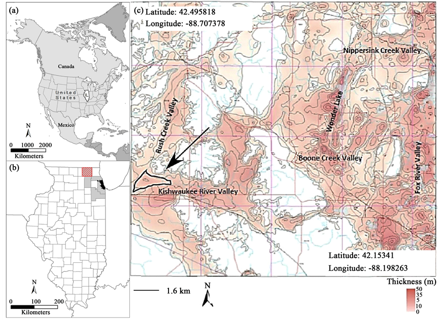
Figure 1. (a) Location of Illinois within the USA; (b) McHenry County, Illinois (gray with red diagonal lines) is the northwest collar-county for the Chicago metropolitan area (black). The latitude and longitude for the northwest corner of the county are: 42.495818 and −88.707378, respectively; (c) Surficial sand and gravel aquifer isopach map for McHenry County. The model area (outlined in black) occurs at the confluence of the Kishwaukee River Valley and the Rush Creek Valley. (Modified from [23] ).
By 2030, the population is projected to grow to more than 10 million [7] . The majority of the population growth is occurring in the collar-counties of Kane, McHenry, and Will (Figure 1), where the area has experienced a 46% increase in residential land use between 1970 and 1990 [8] , and the population is expected to increase 75 and 115 percent by 2030 [7] . With a population that increased from 35,000 in 1930 to 303,990 in 2005, McHenry County has experienced the fastest growth of any county in Illinois [9] [10] . In 2050, the population for McHenry County is projected at 589,000, a 94 percent increase from 2005 [11] . Growth in water demand within the Chicago Metropolitan area, together with declining water levels in deep bed rock wells and strictly regulated use of Lake Michigan water have led to a regional awareness of the need for science-based, sustainable water supply management.
McHenry County is unique compared to the other collar-counties in that all of its water is supplied from groundwater, with about 75% of its groundwater supply coming from shallow sand and gravel aquifers [12] [13] . Most of the groundwater withdrawn has historically been pumped from shallow wells screened in sand and gravel aquifers within 30 meters of land surface [12] . Dziegielewski and Chowdhury [11] estimated 2005 groundwater withdrawals in McHenry County amounted to 148,000 m3/day, a three-fold increase from 1964 [14] . By 2030, average annual water withdrawals will double to 256,000 m3/day, and by 2050 increase by another 30,000 to 231,000 m3/day [9] . Roughly 2% of the water withdrawn is used for irrigation and agriculture [14] , which account for 75% of the land-use in McHenry County [15] .
In response to the accelerated population growth and withdrawals of groundwater, Meyer et al. [14] simulated the effects of public water withdrawal on the shallow and deep aquifer systems of the northeastern Illinois region, including McHenry County in an attempt to predict future drawdown scenarios. Over 8700 wells were represented in drought scenarios showing drawdown levels in the shallow aquifer ranging from 0 to 10 meters and being predominantly located in areas of municipal withdrawal for public use. They concluded that extensive pumping could result in reductions of natural groundwater discharge, thus affecting base flow levels in streams and lakes.
This in turn has led to recognition that a better understanding of the surficial geology and shallow aquifer systems is necessary in order to implement sustainable management practices, specifically the role of irrigation wells. The objective of this paper is to better understand the effects of high-capacity irrigation wells on a surficial sand and gravel aquifer. While the population of McHenry County is expanding, there still exists a vibrant agricultural industry in the western portion of the county. Within the Kishwaukee River Valley, the surficial sand and gravel aquifer is heavily used to meet agricultural demands. A more complete awareness of the groundwater flow patterns in this aquifer and of the potential consequences of pumping will lead to more informed water-management policies. In order to gain a better understanding of the effects of pumping, a steady- state groundwater flow model was constructed using MODFLOW to simulate the current pumping regime and to simulate the effects of different drought scenarios.
2. Materials and Methods
2.1. Site Description
The project focuses on the surficial sand and gravel aquifer at the intersection of the Kishwaukee River Valley and Rush Creek Valley (Figure 1). This project focuses on the effects of high-capacity irrigation wells located in the river valley, screened in the surficial drift sand, and gravel aquifer. As the land use is primarily agricultural, no municipal water wells are located within the model domain.
The Kishwaukee River is located in a paleo-valley of bedrock that has been filled with glacial sediments. The succession of glacial sediments deposited in this valley in recent stages of glaciation host the surficial drift aquifer and many other units. Prior to the Quaternary Period, streams and rivers dissected the bedrock landscape and produced a paleo-topography that is similar to the driftless area 100km to the west. During the subsequent glacial periods, further modification of the valleys occurred by means of glaciers, glacial outwash, and melt-water rivers [12] . In concert with the erosion, these valleys were also being filled in with glacial outwash sediments [16] . Glacial sediments such as sand, gravel, diamicton and clay were deposited in these bedrock valleys and serve as aquifers in McHenry County [15] [17] . Studies of Quaternary materials in McHenry county date back to the 1960’s and explore different facets such as sand and gravel resources [18] [19] , groundwater [12] [17] [20] , general stratigraphy [21] and glacial history [12] [22] . More recently, groundwater investigations have been completed focusing on local aquifers [23] as well as simulation modeling and potentiometric surface mapping in McHenry County [14] .
Within a regional hydrogeological context, four major aquifer systems are present. These systems can be divided into bedrock aquifers and major sand and gravel aquifers. While minor sand and gravel aquifers do exist, the scope of this project does not warrant their discussion. In McHenry County, the lowermost system present is comprised of Silurian-Ordovician bedrock aquifers that can be over 60 meters below the land surface. In eastern McHenry County, the bedrock aquifer is used for domestic and municipal wells. The bedrock aquifers are an important aspect in groundwater interactions and are often in hydraulic connection with the overlying basal drift aquifer near the bedrock/basal drift interface. The basal drift aquifer is comprised mostly of sand and gravel deposits that were associated with glacial meltwater deposition. Given the landscape at the time of deposition, most sediments filled lowlands and bedrock valleys. These aquifers are usually in direct contact with the bedrock and their thickness is generally less than 10 meters but can exceed 30 meters in some areas. The basal aquifer is utilized for both domestic and municipal water supply in the county. The Pearl-Ashmore aquifer is an important water resource in McHenry County for both municipal and domestic withdrawal. The sediments composing the aquifer are associated with the retreat of Illinois-Episode deposits and the advance of Wisconsin Episode glaciation. Typical of outwash sediments, the Pearl-Ashmore is composed of coarse sands and gravels and may include fine to medium sands. Thickness is variable ranging from less than 10 meters to over 30 meters but is thin or non-existent in the study areas of this project. The uppermost aquifer in this succession is the surficial drift aquifer. Not unlike the other aquifers in the area, it is composed of sand and gravel deposits that are often quite shallow and exposed at the surface. Given its composition is from meltwater streams during the Wisconsin Episode depositing sediments, the surficial aquifer is often located in glacial meltwater valleys, which are represented by the modern alluvial valleys in McHenry County. Groundwater within the aquifer discharges to the Kishwaukee River [14] . Thickness of the aquifer ranges from 1 meter along valley edges to over 36 meters in the valley. Utilization of this aquifer is widespread and supplies water for domestic, municipal, and agricultural needs. Specifically, in the Kishwaukee River Valley, large amounts of water are withdrawn from the aquifer for agricultural use, primarily irrigation.
2.2. Conceptual Model
The aquifer system being studied is referred to as the surficial drift aquifer in McHenry County [23] . The unconfined system is composed of various layers of high-conductivity glaciofluvial outwash sediments that have been deposited in the Kishwaukee River Valley (Figure 2). Underlying these units are overlapping layers of both high and low hydraulic conductivity (K) sediments from the previous glacial episodes. The model domain is defined by the Kishwaukee River to the south, Rush Creek, which trends southwest-northeast on the west portion of the boundary, and a constant head boundary to the north, which connects the Kishwaukee River and Rush Creek (Figure 1 and Figure 2). The model domain was divided into four layers based upon the hydrostratigraphy. The three upper hydrostratigraphic units consist of alluvium (Layer 1), sand and gravel (Layer 2), and
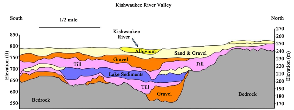
Figure 2. Glacial stratigraphy within the Kishwaukee River Valley. Cross-section is a south-north orientation. Modified from [23] .
gravel (Layer 3). Layer 4, representing a combination of the underlying sediment comprised of low K units including lenses of till, lake sediments, and bedrock, was designated as a separate from the units above. Each layer was assumed to be homogeneous and isotropic. Thicknesses of these layers are variable, especially outside the model domain. Layer 1 is about 5 meters thick in this area. Layer 2 ranges from up to 18 meters, but is absent in some areas. Layer 3 ranges from 0 - 20 meters. The underlying Layer 4 ranges from 60 to 80 meters in the model domain. Hydraulic conductivity values for each layer were estimated from the pumping test data collected, lithological descriptions, and reported values [14] [23] . Given the desire for the underlying low conductivity unit to transition into a no-flow boundary, Layer 4 was assigned an initial K value of 3x10⁻⁸ m/s. Layer 3 represents the gravel lens,which hosts the screened interval for irrigation wells in the area, and is the most transmissive zone with aK value of 3.5 × 10⁻² m/s. Layer 2 is slightly more diverse in its composition (sand and gravel), resulting in an initial K value of 3.5 × 10⁻³ m/s. The uppermost unit in this sequence is a combination of alluvium in the river valley along with the terraces found on the northern extent of the model domain. Given the fingering of the different lithologies, a K value of 3.0 × 10⁻⁴ m/s was assigned. Based upon a mean precipitation value of 0.91 meters per year for McHenry County [24] and adjusted for evapotranspiration, 2.5 × 10⁻⁴ m/day was established as the recharge values for Layer 1 of the model. The recharge rate is consistent with other groundwater recharge rates used for the Chicago area, which are estimated to range between 1.4 × 10⁻⁴ m/day to 8.2 × 10⁻⁴ m/day [14] [25] [26] .
The boundary conditions were assigned based on available model domain and hydrologic condition information that was available. The Kishwaukee River bounds the model to the south and is defined as a constant head boundary. In a similar approach, Rush Creek defines the western edge of the domain. These assigned values were determined by interpreting topographic maps at the upstream and downstream extents of these boundary conditions to as certain head values based upon the elevations and evaluating the stability of the stage for the Kishwaukee River. The bedrock, which houses the valley, rises steeply nearing the land surface as one travels northward from the Kishwaukee River (Figure 1 and Figure 2). Since the exact flux between the bedrock and the sediments in the valley is unknown, a constant-head boundary along the northern edge of the domain was employed. To help establish the boundary conditions for the local model, an analytical element model was developed in GFLOW [27] . Analytical element models are often developed as screening models for a fast hydrologic analyses of an area [28] [29] or to provide boundary conditions and simulate the flow system for extraction into a local three-dimensional model [30] . The GFLOW model simulated a contour representing the 239 m total head contour running parallel to the northern valley, which is consistent with the results of Meyer et al. [14] ; this contour served as a constant-head value for the northern edge of the domain.
2.3. Model Setup
A groundwater flow model was constructed to understand the cumulative effects of the irrigation wells in this region and how different climatic scenarios alter drawdown. The numerical model was established from the conceptual model. Simulations were created to examine steady-state flow, assuming constant recharge and steady-state withdrawal from the irrigation well(s). The initial model examined drawdown from one irrigation well screened within Layer 3 (gravel) at a depth of 18 meters. The rate of withdrawal from the well was 3 m3/min, which is based upon pumping rates provided by farmers in the area.
The groundwater flow model was developed using MODFLOW [31] . Following the MODFLOW development, MODPATH [31] [32] was used to delineate capture zones for each respective well. Reverse particle tracking was utilized for each individual well. After running the MODFLOW simulation, particles were assigned in a circular pattern around each well, and a reverse particle tracking analysis was computed. Particle tracking analysis provides visualization of the travel route and point of origin for the water acquired by a well, revealing their capture zones.
Layer elevations for the tops of the four units, described previously, were obtained from a regional-scale, 3-D model of McHenry County [23] . These layers were imported from ESRI ArcGIS into Groundwater Vistas as shape-files. Aquifer parameters and boundary conditions, as presented in the conceptual model, complete the model development.
2.4. Calibration
Limited data exist to calibrate the model. One set of data is a pumping test conducted using the irrigation well and an observation well located 61 meters from the irrigation well. While limited, the data allowed for calibration and adjustment of the parameters. The constant-head values for the boundaries and K values for the layers were each individually adjusted from their original values to best simulate baseline elevation head values at the pumping well (Table 1). The northern reaches of the model where the bedrock rises steeply in elevation proved the most difficult area to assign head elevations due to the geometry of the units; however, final placement and values agreed with the regional GFLOW model and with the data from Meyer et al. [14] . Hydraulic conductivity values were adjusted for all layers. The upper three layers were modified due to the heterogeneous nature of the units, and therefore possible variation in conductivities. Changes made to the hydraulic conductivity values typically did not result in significant change in the simulated head. However, the lowermost unit was only slightly adjusted in order to simulate very low flow. Once calibrated, MODPATH was applied to generate a visualization of the capture-zone for the irrigation well (Figure 3).
2.5. Scenarios
Following the initial model and calibration, six (6) additional scenarios were simulated in an attempt to understand the system’s response to pumping under different conditions. Well records indicate the presence of four additional wells in the study area that are screened within the aquifer system. Locations of the wells were confirmed using Google Earth and identifying irrigation circles. The four (4) wells were added to the model domain. Based upon the geology and core logs, we assumed that all wells located in the river valley are screened the gravel zone, the most transmissive and productive zone, represented by Layer 3. The rate of pumping was assumed to be the same rate as the original irrigation well. Scenario 1 represents all five wells in the Kishwaukee River Valley pumping at 3 m3/min under normal recharge conditions to represent the base conditions. The next five scenarios were an attempt to model different degrees of drought conditions and were chosen to illustrate a stepwise progression of conditions (Table 2). Each simulation included a progressive decrease in recharge by 10% coupled with an increase in pumping rate by 10%. Historical stream gauge data for the Kishwaukee River (USGS station 0538500 and USGS station 05438170) revealed that stream levels remain constant, even in times of drought. Therefore, only the final simulation includes a lowering of the constant head boundary representing the Kishwaukee River (0.15 meters lower) in conjunction with a 50% decrease in recharge and 50% increase in pumping.
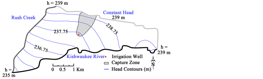
Figure 3. Model domain with Initial model results for the one irrigation well scenario. The results provide the simulated potentiometric surface and the capture zone.

Table 1. Initial and final values for model parameters.
Table 2. Recharge and rate of well pump age for the simulated scenarios.
A statistical analysis of cell-by-cell head values between the model runs was completed. Each analysis compared the head levels in each cell of Scenario 1 (normal recharge and pumping rates) against the head levels of the same cells in the subsequent Scenarios 2 through 6. Paired difference tests, with an α = 0.05, were used to compare how the head values change between each individual scenario and Scenario 1.
3. Results and Discussion
Scenario 1 generated baseline head distribution and capture zone areas that were used for comparison with the other scenarios (Figure 4 and Table 3). Compared to the initial simulation, one irrigation well, the Scenario 1 results are visually similar. Exception includes migration of the 237.75 m potentiometric surface contour to the north and the eastward migration of the 238.75 contour. Movement of both lines is the result of the additional pumping and decrease in elastic storage within the gravel aquifer. The five wells generated four capture zones: West; Middle; and two East zones that represent the three eastern wells. While all wells draw water from the northern boundary, the eastern two wells draw from the Kishwaukee River. In total, the wells capture water from 1.55 km2.
Contours of the potentiometric surface and the capture zone delineations for each scenario provide additional understanding of how the pumping regime could alter flow patterns in each modeled scenario. As the recharge drops and pumping rates increase, more change is noticed in the contours. The potentiometric contours show localized cones of depression around each well with upgradient migration of the equipotential lines. Scenario 1 shows more separation between capture zones of each respective well and a relatively small portion being drawn from the Kishwaukee River. Beginning with Scenario 2, the capture zones for the three eastern wells merge. The combined East zone increases in size and develops a larger contact area with the Kishwaukee River (Figure 4).
In regards to the capture zone analysis, the diminishing width of the surficial drift aquifer in the eastern area of the model domain results in less water available to each well, therefore, they must draw more from the Kishwaukee River to meet the pumping demand. The cumulative effect of the higher concentration of wells in this area increases the capture zone sizes (Table 4). Overall, capture zone area increases 32% from 1.55 km2 to 2.05 km2, which is smaller than the combined decrease in recharge and increase in pumping.
The results of the statistical analysis performed between model runs are represented in Table 3. The p-Value can be compared between each different scenario to analyze whether or not the change in head values in these cells is statistically significant. With Scenarios 2 and 3, the head values throughout the model are not statistically different from in Scenario 1. Only when recharge is dropped 30% and pumping is increased 30% (Scenario 3) is significant change witnessed, with the most recognizable changes occurring in the Scenario 6. The statistical analysis supports the visual representation of the flow patterns.
Given the period and data available, the conditions modeled were considered appropriate. However, the simulations are not a perfect representation of actual conditions, specifically in regards to those simulating drought and increased pumping. Typically, drought conditions show a decrease in precipitation, which in turn is assumed to lead to an increase in pumping. This respective increase is difficult to quantify and therefore may not be modeled in a manner most representative of actual conditions. Lastly, this simulation provides results for steady-state conditions. It is difficult to determine then what the effects of extended drought and increased pumping over longer time-steps will have on the shallow aquifer system.
Table 3. Results of statistical analysis on head levels compared with Simulation 1.
Table 4. Capture zone areas.

Figure 4. Potentiometric surfaces for Layer 2 for each of the six Scenarios with multiple wells. Capture zone are represented by gray areas. p-values are representative of Layer 2. (a) Scenario 1; (b) Scenario 2; (c) Scenario 3; (d) Scenario 4; (e) Scenario 5; (f) Scenario 6.
4. Conclusions
The groundwater flow model can be an appropriate tool in assessing the impacts of high-capacity irrigation wells in local unconfined aquifers of McHenry County. This project focused on the quantitative assessment of these wells, and gave insight into the sustainability of the aquifer given the current conditions. However, this research also adds to the collective knowledge about unconfined, unconsolidated aquifer systems and anthropogenic impacts. Given the widespread nature of these aquifers throughout the Midwest and their prolific use, the approach taken in this research project may be a simple and effective way to understand sustainable use in similar aquifers.
The groundwater flow model was developed to understand the singular and cumulative effect of high-capacity irrigation wells located in the Kishwaukee River Valley, specifically wells screened and withdrawing from the surficial drift aquifer. The results presented in Figure 4 show potentiometric surface contours and capture zones for each respective model run. It is important to note that while there are noticeable changes in the contour patterns, the overall flow pattern is not significantly altered by the changes in recharge and pumping rates. Local change in the contours is present around the wells, but does not extend to great lengths beyond their pivot radius. More change can be seen on the eastern side of the model area as compared to the west. This is hypothesized to be a result of the diminishing width of the surficial aquifer as it extends northward from the Kishwaukee River on the eastern side. The fact that the contours are not as altered on the west side is hypothesized to be the effect of the confluence of the Kishwaukee River and Rush Creek.
The model and scenarios suggest: 1) the glacial materials within the valley allow for recharge and have enough storage to accommodate changes of 20% in terms of recharge and pumping. 2) In the event of less recharge, the area should be able to accommodate current withdrawals, but even with greater withdrawals, little impact on the aquifer will be observed. As the eastern wells draw from the Kishwaukee River, impacts may be seen on river stage; however, that was not an objective of this model. The results of the scenario reveal the influences of using constant head conditions along the boundaries, as the constant head conditions dictate the distribution of the equipotential lines. Changes in the leakage, potential flow from the bedrock aquifer, would alter the presented results and need to be considered in future work. As the scenarios only examined steady-state, the study did no climate variability over multiple years and what cumulative effects could occur.
Overall, scenarios 4, 5, and 6 show a statistically significant difference in equipotential lines as compared to Scenario 1. Although forecasts predict and increase in precipitation [2] , a decrease in recharge [5] may occur as more precipitation falls during the winter. Winter precipitation will not infiltrate and will runoff more easily. The model shows the system is capable of sustaining a decrease in recharge of 20%, suggesting current policies and practices are sustainable. Because of the county’s rapid population growth, however, ground-water withdrawals have increased. The need to accommodate future growth in population must be balanced with concerns over resource conservation, environmental protection, and public health [20] .
The growth in population has resulted in an increase in water usage; from 1980 to 1992, water use increased about 27 percent (Kirk et al., 1982; Avery, 1999). With predicted population growth, Dziegielewski et al. (2004) projected an increase in water demand of 20 percent between 2005 and 2025. Because Illinois has legal constraints on withdrawals from Lake Michigan (capped at 3200 cubic feet/second by the U.S. Supreme Court in 1967) and withdrawals from deep bedrock aquifers exceed estimated recharge rates, shallow bedrock and overlying sand and gravel aquifers are expected to be the main sources of water to meet increased demand. Groundwater withdrawn from these shallow aquifers can be replaced by natural processes at considerably higher rates than is possible from deep bedrock aquifers [33] , which may lead to increased municipal water withdrawals that will impact the outcomes of the presented model.
Cite this paper
Logan C. Seipel,Eric W. Peterson,David H. Malone,Jason F. Thomason, (2016) Role of Multiple High-Capacity Irrigation Wells on a Surficial Sand and Gravel Aquifer. Journal of Geoscience and Environment Protection,04,43-53. doi: 10.4236/gep.2016.45005
References
- 1. Pryor, S.C., Scavia, D., Downer, C., Gaden, M., Iverson, L., Nordstrom, R., Patz, J. and Robertson, G.P. (2014) Chapter 18: Midwest. In: Melillo, J.M., Richmond, T.C. and Yohe, G.W., Eds., Climate Change Impacts in the United States: The Third National Climate Assessment, Publisher, Location, 418-440.
- 2. Pryor, S. and Barthelmie, R. (2013) The Midwestern United States: Socioeconomic Context and Physical Climate. In: Pryor, S.C., Ed., Climate Change in the Midwest: Impacts, Risks, Vulnerability, and Adaptation, Indiana University Press, Bloomington, IN, 12-47.
- 3. Pryor, S., Barthelmie, R. and Schoof, J. (2013) High-Resolution Projections of Climate-Related Risks for the Midwestern USA. Climate Research, 56, 61-79.
http://dx.doi.org/10.3354/cr01143 - 4. Pryor, S., Kunkel, K. and Schoof, J. (2009) Did Precipitation Regimes Change during the Twentieth Century? In: Pryor, S.C., Ed., Understanding Climate Change, Indiana University Press, Bloomington, IN, 100-112.
- 5. Barry, R., Armstrong, R., Callaghan, T., Cherry, J., Gearheard, S., Nolin, A., Russell, D. and Zöckler, C. (2007) Snow Global Outlook for Ice and Snow. United Nations Environmental Programme, Birkeland, 39-62.
- 6. Wilhite, D.A. and Glantz, M.H. (1987) Understanding: The Drought Phenomenon: The Role of Definitions. In: Wilhite, D.A., Easterling, W.E. and Wood, D.A., Eds., Planning for Drought: Toward a Reduction of Social Vulnerability, Westview Press, Boulder, CO, 11-30.
- 7. Northeastern Illinois Planning Commission (NIPC) (2007) Northeastern Illinois Planning Commission Endorsed 2030 Forecasts Revised. Northeastern Illinois Planning Commission, Chicago, IL.
- 8. Northeastern Illinois Planning Commission (NIPC) (1996) Strategic Plan for Land Resource Management. Northeastern Illinois Planning Commission, Chicago, IL.
- 9. McKinney, C. (2011) Update on Water Studies Groundwater Protection Program. Division of Water Resources, County of McHenry.
- 10. U.S. Census Bureau (2000) Census of Population. U.S. Census Bureau, Suitland, MA.
- 11. Dziegielewski, B. and Chowdhury, F.J. (2008) Regional Water Demand Scenarios for Northeastern Illinois: 2005-2050. Department of Geography and Environmental Resources, Southern Illinois University, Project Completion Report Prepared for the Chicago Metropolitan Agency for Planning.
- 12. Curry, B.B., Berg, R.C. and Vaiden, R.C. (1997) Geologic Mapping for Environmental Planning. McHenry County, Illinois, Illinois State Geological Survey, Champaign, IL, Circular 559.
- 13. Hwang, H.-H., Panno, S.V., Hackley, K.C. and Walgren, D. (2007) Chemical and Isotopic Database for McHenry County Study on Groundwater Quality and Land Use. Illinois State Geological Survey, Champaign, IL, Open File Series 2007-6.
- 14. Meyer, S.C., Lin, Y.-F., Abrams, D.B. and Roadcap, G.S. (2013) Groundwater Simulation Modeling and Potentiometric Surface Mapping. McHenry County, Illinois, Illinois State Geological Survey, Champaign, IL, Contract Report 2013-06.
- 15. Berg, R.C., Curry, B.B. and Olshansky, R. (1999) Tools for Groundwater Protection Planning: An Example from McHenry County, Illinois, USA. Environmental Management, 23, 321-331.
http://dx.doi.org/10.1007/s002679900189 - 16. Ritzi Jr., R.W., Jayne, D.F., Zahradnik Jr., A.J., Field, A.A. and Fogg, G.E. (1994) Geostatistical Modeling of Heterogeneity in Glaciofluvial, Buried-Valley Aquifers. Ground Water, 32, 666-674.
http://dx.doi.org/10.1111/j.1745-6584.1994.tb00903.x - 17. Carlock, D.C., Thomason, J.F., Malone, D.H. and Peterson, E.W. (2016) Stratigraphy and Extent of the Pearl-Ashmore Aquifer, Mchenry County, IL, USA. World Journal of Environmental Engineering, 4, 6-18.
- 18. Anderson, R.C. and Block, D.A. (1962) Sand and Gravel Resources of McHenry County, Illinois, State of Illinois. Department of Registration and Education, Division of the State Geological Survey Circular 336.
- 19. Specht, S. and Westerman, A. (1976) Geology for Planning in McHenry County, v. Ill: Illinois State Geological Survey.
- 20. Meyer, S.C. (1998) Ground-Water Studies for Environmental Planning. McHenry County, Illinois, Illinois State Water Survey, Champaign, IL, Contract Report 630
- 21. Berg, R.C., Kempton, J.P., Follmer, L.R., McKenna, D.P. and Krumm, R.J. (1985) Illinoian and Wisconsinan Stratigraphy and Environments in Northern Illinois: The Altonian Revised. Illinois State Geological Survey, Champaign, IL.
- 22. Seipel, L.C., Thomason, J.F., Malone, D.H. and Peterson, E.W. (2015) Surficial Geology of Garden Prairie 7.5-Minute Quadrangle, Boone and McHenry Counties, Illinois Illinois State Geological Survey, Illinois State Geological Survey.
https://www.isgs.illinois.edu/maps/isgs-quads/surficial-geology/garden-prairie - 23. Thomason, J.F. and Keefer, D.A. (2013) Three-Dimensional Geologic Mapping for McHenry County. Illinois State Geological Survey, Champaign, IL, Contract Report.
- 24. Calsyn, D.E. (2001) Soil Survey of McHenry County Natural Resources Conservation Service.
- 25. Roadcap, G.S., Cravens, S.J. and Smith, E.C. (1993) Meeting the Growing Demand for Water: An Evaluation of the Shallow Ground-Water Resources in Will and southern Cook Counties, Illinois. Illinois State Water Survey, Champaign, IL, ISWS RR-123.
- 26. Arnold, J.G., Muttiah, R.S., Srinivasan, R. and Allen, P.M. (2000) Regional Estimation of Base Flow and Groundwater Recharge in the Upper Mississippi River Basin. Journal of Hydrology, 227, 21-40.
http://dx.doi.org/10.1016/S0022-1694(99)00139-0 - 27. Haitjema, H.M. (1995) Analytic Element Modeling of Groundwater Flow. Academic Press, San Diego, CA.
- 28. Hunt, R.J. (2006) Ground Water Modeling Applications Using the Analytic Element Method. Ground Water, 44, 5-15.
http://dx.doi.org/10.1111/j.1745-6584.2005.00143.x - 29. Feinstein, D., Dunning, C., Hunt, R.J. and Krohelski, J. (2003) Stepwise Use of GFLOW and MODFLOW to Determine Relative Importance of Shallow and Deep Receptors. Ground Water, 41, 190-199.
http://dx.doi.org/10.1111/j.1745-6584.2003.tb02582.x - 30. Hunt, R.J., Anderson, M.P. and Kelson, V.A. (1998) Improving a Complex Finite-Difference Ground Water Flow Model Through the Use of an Analytic Element Screening Model. Ground Water, 36, 1011-1017.
http://dx.doi.org/10.1111/j.1745-6584.1998.tb02108.x - 31. McDonald, M.G. and Harbaugh, A.W. (1988) A Modular Three-Dimensional Finite-Difference Ground-Water Flow Model. United States Geological Survey, Washington DC.
- 32. Pollock, D.W. (1989) Documentation of Computer Programs to Compute and Display Pathlines Using Results from the U.S. Geological Survey Modular Three-Dimensional Finite-Difference Ground-Water Flow Model. Denver, CO, Open-File Report 89-381.
- 33. Kelly, W.R. and Wilson, S.D. (2008) An Evaluation of Temporal Changes in Shallow Groundwater Quality in Northeastern Illinois Using Historical Data. Illinois State Water Survey, Champaign, Illinois, Scientific Report 2008-01.
NOTES

*Corresponding author.