American Journal of Industrial and Business Management
Vol. 3 No. 3 (2013) , Article ID: 33729 , 12 pages DOI:10.4236/ajibm.2013.33035
Retail Price Optimization from Sparse Demand Data
![]()
1School of Engineering and Mathematical Sciences, City University London, London, UK; 2Cass Business School, City University London, London, UK.
Email: pjt3.michaelmas@gmail.com
Copyright © 2013 Philip Thomas, Alec Chrystal. This is an open access article distributed under the Creative Commons Attribution License, which permits unrestricted use, distribution, and reproduction in any medium, provided the original work is properly cited.
Received March 24th, 2013; revised April 24th, 2013; accepted May 24th, 2013
Keywords: Optimal Price; Monopoly; Monopolistic Competition; Oligopoly; Sparse Demand Data; Retail
ABSTRACT
It will be shown how the retailer can use economic theory to exploit the sparse information available to him to set the price of each item he is selling close to its profit-maximizing level. The variability of the maximum price acceptable to each customer is modeled using a probability density for demand, which provides an alternative to the conventional demand curve often employed. This alternative way of interpreting retail demand data provides insights into the optimal price as a central measure of a demand distribution. Modeling individuals’ variability in their maximum acceptable price using a near-exhaustive set of “demand densities”, it will be established that the optimal price will be close both to the mean of the underlying demand density and to the mean of the Rectangular distribution fitted to the underlying distribution. An algorithm will then be derived that produces a near-optimal price, whatever the market conditions prevailing, monopoly, oligopoly, monopolistic competition or, in the limiting case, perfect competition, based on the minimum of market testing. The algorithm given for optimizing the retail price, even when demand data are sparse, is shown in worked examples to be accurate and thus of practical use to retail businesses.
1. Introduction
The markets faced by retailers in different sectors may span the range of market categories from perfect competition, through oligopoly, monopolistic competition to monopoly. But the problem of setting the optimal price faces retailers in all market categories. Selling to multiple customers, they need to offer a price that is common to all. This study appeals to standard economic theory to help illuminate the position of the retailer as he uses whatever information is available to him in order to set the price of each product so as to maximize his profit. The end point will be an algorithm for setting the price of a product that will be close to the optimum, whatever the market conditions prevailing, based on the minimum of market testing.
Finding the price to maximize profit would be relatively easy if the retailer knew the maximum price acceptable to each of his customers interested in buying the product. Any given price would imply that the retailer would gain income from all those whose maximum acceptable price (MAP) lay above this level. His turnover having now been decided, the retailer could then calculate first his costs and then, by subtraction, his profit. Applying the same procedure to all or a selection of prices would quickly show the retailer what price he should set to generate the highest profit.
Obtaining the necessary information on the MAP for each customer could be attempted via a market survey. Normalizing the results by dividing by the number taking part would give a probability distribution for MAP, which may be called the “demand density” for compactness. A demand density found in this way would, of course, be subject not only to the inaccuracies associated with any sampling operation but also to those associated with a sample that might be less than perfectly representative. Moreover the survey would need to be applied to each product and repeated at regular intervals. Such a large and ongoing data collection exercise, although feasible in principle, would be impractical to implement.
The alternative, and the approach used here, is to postulate a wide range of possible demand densities, h(p), and then use standard economic theory to investigate the relationship between the optimal price and other central measures of MAP, which may lend themselves to use in a price-optimization algorithm. The restriction on a probability distribution, namely that the area under the curve must be unity, viz. , aids in this process, allowing near-exhaustive testing of possible demand scenarios using a finite number of candidate demand densities.
Two sets of candidate demand densities are used. The first assumes that the MAP is proportional to the ability to pay as measured by post-tax household annual income up to one of a set of percentile levels. The second set consists of the “Double Power” demand density defined in Section 7, with different coefficients locating its mode anywhere between 0 and the highest price that anyone is prepared to pay for the item (normalised to 10 units in the examples considered).
A third, generalized demand density is also considered, namely the Rectangular demand density. It is the demand density assumed by default by economists when they draw a straight-line, downward-sloping demand curve, and it has particular significance because the optimal price and the mean price are the same. The Rectangular is, moreover, the simplest demand density able to fit the mental model of a retailer who knows 1) the lowest price at which he would countenance selling the product and 2) the highest price he could get from his customers before sales became negligible.
The Rectangular demand density may be fitted with good accuracy to demand densities in both of the candidate sets. The matched Rectangular demand density may then be regarded as a proxy for the underlying distribution, a fact that will be exploited in the price optimization algorithm introduced later.
2. The Demand Density Underlying the Conventional Demand Curve
The conventional demand curve may be regarded as a plot of price, p, against the fraction,  , of the target market prepared to pay that price or more [1-3]. It is usual for the marginal revenue and the variable cost to be plotted also, resulting in a diagram similar to Figure 1, in which it is assumed that the variable component of cost is linear. While the conventional demand curve uses the cumulative probability,
  , as one of its axes, there are advantages in recasting
  in terms of its fun-
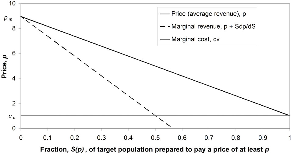
Figure 1. Conventional demand curve.
damental demand density,  , since this fraction is the integral of probability density above price, p:
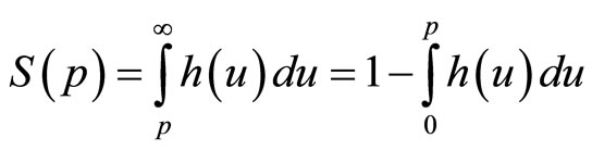 (1)
(1)
where the second development follows from the fact that .
.
Although the same information is carried by S(p) as by h(p), the fact that the former is based on an integration of the latter means that it is a filtered version, so that the detail is more difficult to pick out. Thus the “demand density curve” of h(p) vs. p offers finer discrimination than the conventional “demand curve” of p vs. S(p). A further advantage of the demand density curve is that, as explained in the next Section, it allows the optimal price to be found naturally.
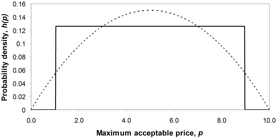
The lesser discrimination inherent in the cumulative probability, S(p), explains why a straight-line approximation to the curve of p vs. S(p) can be used routinely in economics text books, even though such a straight-line demand curve will hold true only when the demand density is Rectangular. For what shows up as a major discrepancy from uniformity in the graph of h(p) vs. p reduces to a minor deviation in the graph of S(p) vs. p. For example, in the case where a symmetrical underlying demand density is approximated by a Rectangular demand density, it is clear from comparing Figures 2(a) and (b) that the difference between the two distributions becomes much less marked when the conventional demand curve is used.
Monopoly is the simplest of the selling situations where multiple customers are involved, since the retailer need be concerned only with the reactions of customers and not of other suppliers. While results as derived in Sections 3 to 9 may be understood in this light, it will be shown in Section 10 that the results will apply equally to all the basic forms of interaction between the retailer and his customers:
• monopoly
• oligopoly
• monopolistic competition as well as, in their limiting form, to perfect competition.
3. Mathematico-Economic Model of Profit Maximization
A retailer will, in general, face a differentiated market, with different people being prepared to pay a different maximum price for the same good, as illustrated in the demand density curve. The term, “uniconsumer”, might be used to denote a consumer prepared to buy one but only one item if the price is right. Then a person, a “mul-
 (a)
(a)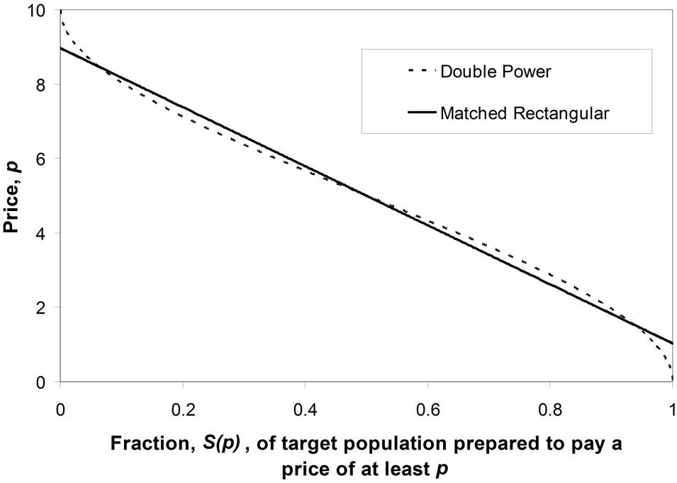 (b)
(b)
Figure 2. Approximating a symmetrical probability density for demand by a Rectangular distribution. (a) Comparison of demand density curves; (b) Comparison of demand curves.
ticonsumer”, who will buy more than one item if the price is right may be represented, as far as his economic behaviour is concerned, as multiple, identical uniconsumers. Suppose that the retailer sets the price at some value, p. The good will be bought by the fraction of uniconsumers, S(p), with a MAP at or above p, as given by Equation (1).
In the rest of the paper we shall use the word, “consumer”, in place of the more exact “uniconsumer”, simply to make it less cumbersome to read. The total number of sales will be NS(p), where N is the size of the population of consumers under consideration. Given a common price, p, the retailer’s income will be NpS(p). Following a standard economic model widely used in business, it will be assumed that the retailer’s costs comprise a linear variable cost,  (£ per item), and a fixed cost independent of the number of items sold,
  (£). His profit,
  , will be the difference between income and costs:
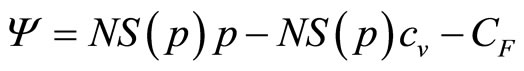 (2)
(2)
The retailer will seek to maximize this profit, which, for a constant size of target population, N, is equivalent to maximizing the average profit per consumer, :
:
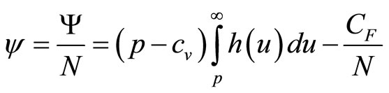 (3)
(3)
where use has been made of Equation (1) in the second step. Since no-one has infinite resources, everyone must have a MAP that lies beneath some maximum conceivable value,  , implying that
 . Hence, we may rewrite Equation (3) as
 (4)
(4)
We may find the maximum value of profit,  , by differentiating Equation (4) with respect to price, p, and then setting
 . At this point,
  , the optimal selling price, which it the price that will generate the retailer the greatest profit. Applying the rules of calculus:
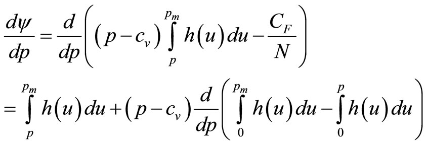 (5)
(5)
Differentiating the contents of the final bracket and setting the whole to zero gives the optimal price as the solution, p, of
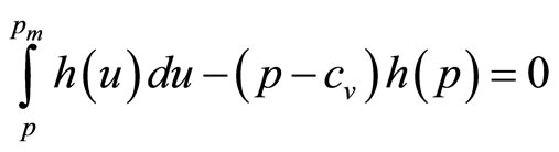 (6)
(6)
4. The Retailer’s Estimate of Demand Density: Sparse Data
The mathematics given in the previous Section provide a way of calculating the optimal price that may be slightly more sophisticated than the method explained in the 2nd paragraph of the Introduction, but they do not get around the fact that solving Equation (6) still requires a knowledge of the demand density, h(p). But in the absence of repeated market surveys, the data available to the retailer are likely to be sparse and fragmentary, in which case he will need to rely on a largely intuitive feel for the demand density characterizing his target market.
Consider now the likely minimum information available to the retailer. We may assume that he will know his variable cost per item, . He will have no interest in selling the item at a price below this level, since sales at a lower price will not make a contribution to offsetting his fixed costs but will, on the contrary, increase his loss. Hence he will regard his target population of consumers as one containing only a negligible fraction for whom the MAP is less than
 . The variable cost per item may then be regarded as defining the lowest price in the retailer’s mental model,
 :
: . (It may be noted that the variable cost,
  , is not a wholly exogeneous cost imposed on the retailer. Its value will reflect choices made by the retailer and those in his supply chain, all of whom will be influenced by perceptions of what the market will bear.)
There are cases where the cost of the good is dominated by fixed costs, and the variable cost per item is essentially zero. Hence the retailer’s mental model may include  as a limiting case. Meanwhile, a knowledgeable retailer should have an idea of the highest MAP,
  , above which his total sales will be negligible: almost nobody will pay more than
 .
.
These two price levels,  and
and , are sufficient on their own to generate for the retailer a simple mental model, g(p), of the true demand density, h(p). The approximating probability density, g(p), will be uniform between
  and
and  and zero elsewhere—a Rectangular distribution. The simple mental model just ascribed to the retailer working with sparse data will generate a straight-line demand curve, as noted in Section 2. Thus it coincides with the default model frequently used by economists when considering the problem of demand.
5. Properties of the Rectangular Demand Density
5.1. Mean, Median and Mode
The Rectangular demand density,  , has the form:
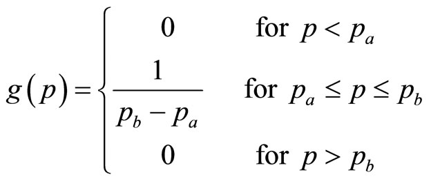 (7)
(7)
The mean value of the MAP,  , is then the weighted average:
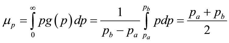 (8)
(8)
Because the Rectangular distribution is symmetrical, the mean and median are equal.
By mathematical convention regarded as unimodal, the Rectangular distribution may be seen as having a mode anywhere in the range, (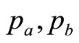 ).
).
5.2. The Optimal Price, p*
Applying Equation (6) with the Rectangular probability density,  , replacing
  and using the equality of the variable cost per unit and the retailer’s lowest MAP of interest,
 :
:
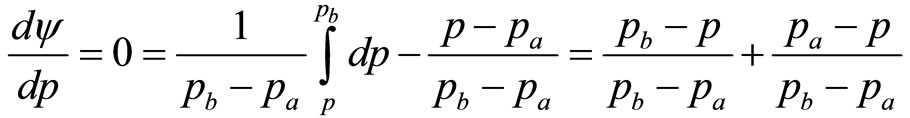 (9)
(9)
So that, denoting the optimal price by p*:
 (10)
(10)
Thus, using the Rectangular demand density likely to be used initially by the retailer as well as by economists in their first consideration of demand, the important result emerges that the optimal price and the mean price will coincide:
 (11)
(11)
Since the mean and median are equal in a symmetrical distribution, it follows also that
 (12)
(12)
where  is the median of the retailer’s Rectangular demand density.
It must be considered unlikely, however, that the true demand curve will be exactly straight, nor, by the same token, will the demand density curve be precisely Rectangular. Hence, while the value,  , may be close to optimal, it will not be the true optimum. To find out how near to the true optimum the mean of the Rectangular distribution is likely to be, we may examine how far it can be made representative of a wide variety of underlying demand densities.
5.3. Matching the Rectangular Demand Density to the Underlying Demand Density
If the true, underlying distribution were known, it would be possible to model the retailer’s intuitive identification of the lower and upper limits of his Rectangular distribution by the mathematical procedure of minimizing the integrated square error between the Rectangular distribution and the underlying distribution. In practice, the underlying distribution is not likely to be known, but a near-exhaustive survey may be made using candidate distributions with characteristics spanning the possible probability space. Once the Rectangular demand density, g(p), has been matched to the underlying demand density, h(p), the mean of g(p), which we shall call the matched Rectangular mean, becomes a property of h(p).
6. Demand Density: Candidate 1, When the MAP Is Proportional to the Ability to Pay
Prima facie, one reasonable assumption is that the MAP is conditioned by, and, in the simplest case, proportional to the ability to pay. Demand density may then be related to post-tax household annual income [4]. It is further supposed that the price of commodities that are needed and obtained by almost everyone in the population will be determined by the attitudes and decisions of those with incomes up to some percentile level, θ. Those with incomes above the  th percentile are then considered to be price-takers for these goods. (For example, very wealthy people may have their shopping done for them, and their less wealthy agents may tend to apply their own personal judgements on what constitutes value for money).
The percentage of people,  , determining the price of each commodity may vary according to commodity, and moreover, that percentage may not be known with any precision. To cope with this situation, we have allowed for
  to take a range of possible percentages, from 51% to 99%. Table 1 gives cumulative probabilities for income; it may be noted that the last column, where
 , is incomplete due to lack of IFS data beyond the 99th percentile.
Figure 3 shows the case for the 85th percentile cohort. (The highest MAP that anyone in the cohort will assign,  , is set to 10 units in each case, a convention that will be followed throughout the paper.) It may be remarked immediately that the distribution shown in Figure 3 is interior unimodal, in the sense that the mode lies strictly within the interval
 .
.
Figure 4 plots the normalised mode, median and mean as well as the optimal price for the underlying distribution, h(p), as well as the mean of the retailer’s matched Rectangular distribution, g(p), versus percentile for all the percentiles listed in Table 1. Clearly the optimal price, based on the underlying distribution, h(p), is distinct from all the other measures. However, both the median and the mean of the underlying distribution, h(p), are reasonable approximations to the optimal price, the mean performing better for lower percentiles, the median
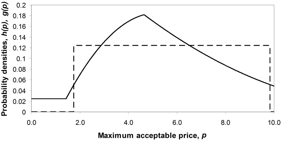
Figure 3. Demand density, h(p), for 85th percentile cohort. Also shown is the matched Rectangular demand density, g(p).
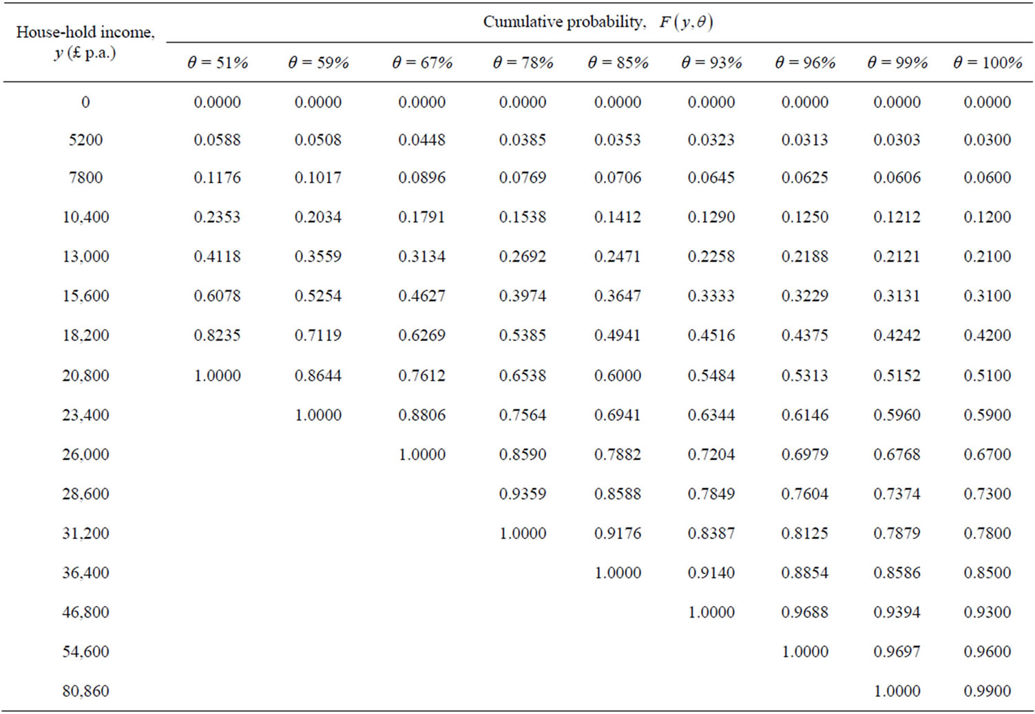
Table 1. UK post-tax household income 2009: Cumulative probability,  , up to the
  th percentile income (equivalised, based on a couple with no children).
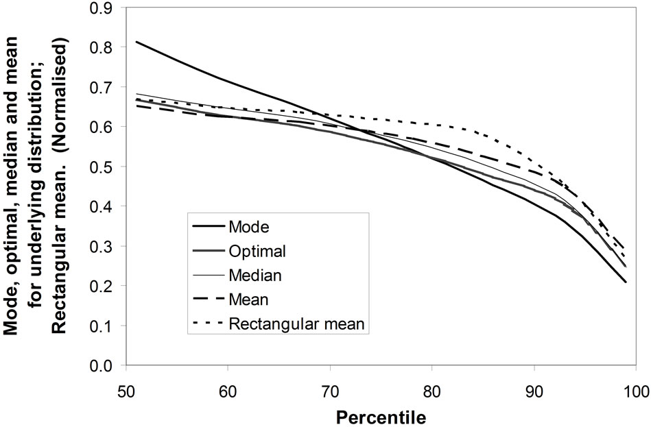
Figure 4. Mode, optimal, median and mean of underlying demand density, h(p); mean of Rectangular demand density, g(p). Plotted versus income percentile.
doing better for percentiles above about 75%. The rootmean-squared error is about 5% for the underlying median and 6% for the underlying mean.
The matched Rectangular mean is a slightly worse approximation to the optimal price for the underlying distribution, being an average of about 10% too high over the range considered, rising to 20% in the worst case of the 85th percentile.
The mode gives a relatively poor approximation to the optimal price. However, it provides a useful way of characterizing the demand density. Figure 5" target="_self"> Figure 5 shows the optimal, mean, and matched Rectangular mean plotted against the mode of the underlying distribution. Larger deviations between the mean and the optimal price are evident when the mode is located centrally in the range.
7. Demand Density: Candidate 2, the “Double Power” Demand Density
The Double Power demand density introduced here is defined on non-negative values of MAP, p, by:
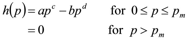 (13)
(13)
where the coefficients, a, b, c and d are non-negative. The Double Power demand density has the desirable property that, through suitable selection of its parameters, a, b, c and d, its mode may be located anywhere between zero and the maximum conceivable value:  , thus ensuring the necessary coverage of the probability space.
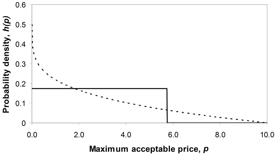
7.1. Mode at the Zero Boundary
The mode lies at the zero boundary,  , when c = 0. The fact that the matched Rectangular demand density has
  implies a zero variable cost:
 . The curve of
  is strictly convex when
 , linear when
  and strictly concave when
 . See Figures 6(a) and (b).
7.2. Mode at the Maximum Boundary, Pm
The mode occurs at the maximum price,  , when b = 0 (except for the limiting case where c is also zero: if
 , the probability distribution becomes uniform
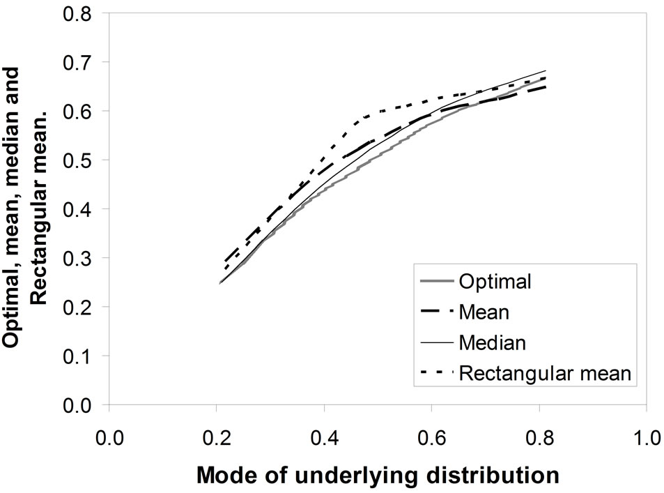
Figure 5. Optimal, mean, median and rectangular mean versus the mode of the underlying distribution.
 (a)
(a)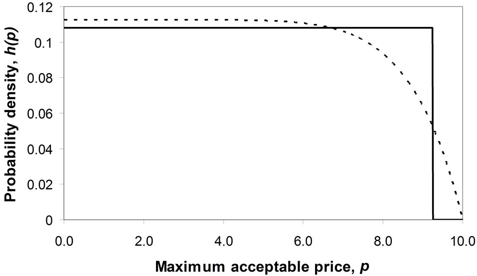 (b)
(b)
Figure 6. Matching a Rectangular demand density to convex and concave Double Power demand densities when the mode is 0.0. (a) Convex Double Power demand density: c = 0, d = 0.25; (b) Concave Double Power demand density: c = 0, d = 8.0.
on (0, ), with no unique mode). The curve of
  is strictly concave when
 , linear when
  and strictly convex when
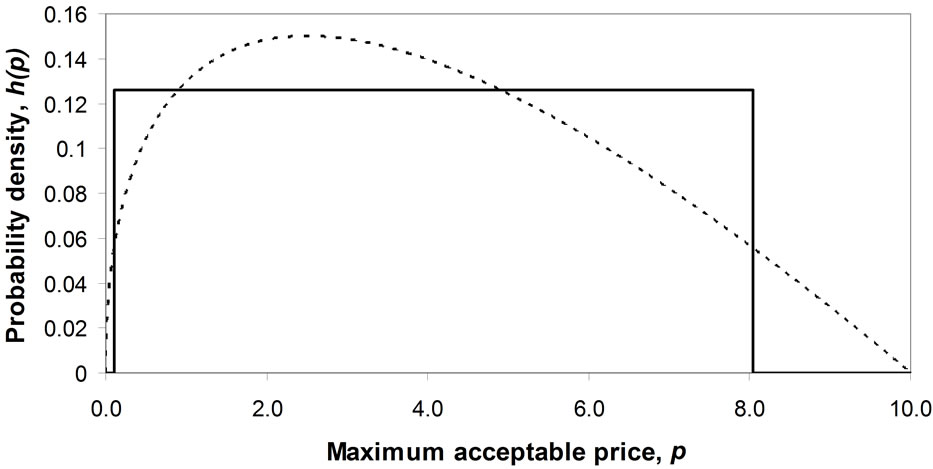
  (Figures 7(a) and (b)).
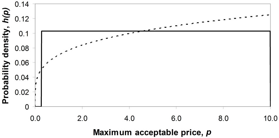
7.3. Mode Strictly Interior
The mode will be strictly interior when the coefficients, a, b, c and d are all positive. See Figure 8. Once c has been set, a suitable selection of d allows the mode to be located anywhere in the range between 0 and , with the mode increasing as d increases.
Figure 8(c), where c = 8 and d = 128, shows also how a high value of the power, c, used in conjunction with a high value of the power, d, can simulate approximately the situation where the effective lowest MAP is above zero–roughly p = 5 in this case. A large majority of population is prepared to pay 5 units or more for the good.
8. Results Using the Double Power Demand Density
8.1. Mode at the Zero Boundary
Figure 9 shows the behaviour of the optimal price, the mean price, the median and the matched Rectangular mean price, as the power, d, is varied from 10−3 to 103. While the optimal is distinct from the other central mea-
 (a)
(a)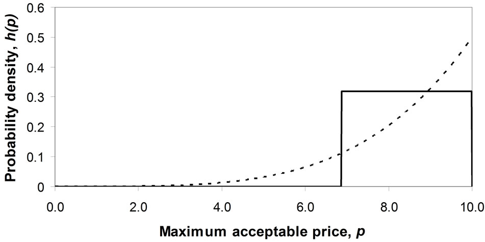 (b)
(b)
Figure 7. Matching a Rectangular demand density to concave and convex Double Power demand densities when the mode takes the maximum value, pm. (a) Concave Double Power demand density: b = 0, c = 0.25; (b) Convex Double Power demand density: b = 0, c = 4.0.
 (a)
(a)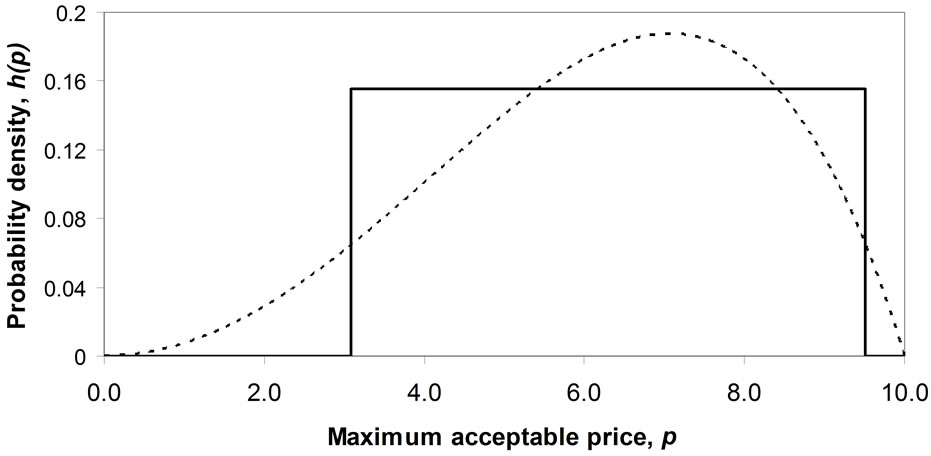 (b)
(b)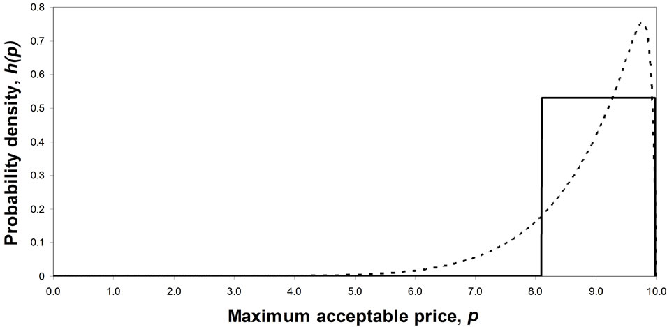 (c)
(c)
Figure 8. Matching a Rectangular demand density to a Double Power demand density with a strictly interior mode. (a) Double Power demand density. c = 1, d = 0.5; (b) Double Power demand density. c = 2, d = 4; (c) Double Power demand density. c = 8, d = 128.
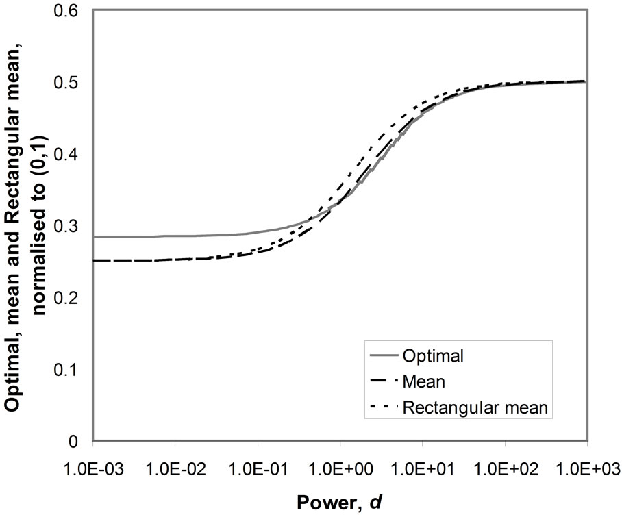
Figure 9. Boundary mode at p = 0. Varying the power, d.
sures, the mean and the matched Rectangular mean are reasonable approximations to it over the whole range, with a maximum error of about 12%.
8.2. Mode at the Maximum Boundary
Figure 10 shows the behaviour of the optimal price, the mean price, the median and the matched Rectangular mean price, as the power, c, is varied from 10-3 to 103. The mean and the matched Rectangular mean show a good correspondence with the optimal over the whole range. The maximum error is about 4%.
8.3. Mode Strictly Interior
Figure 11 shows the optimal price, the mean price and the matched Rectangular mean price against the mode when the parameter, c, is equal to 2. The optimal price is distinct, but each of the other central measures acts as a reasonable approximation to it over the whole range of modes for all the values of c examined. The maximum discrepancy, of about 9%, occurs when the mode is mid-range.

Figure 10. Boundary mode at p = pm. Varying the power, c.
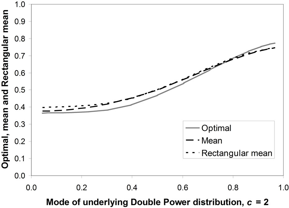
Figure 11. Optimal, mean and Rectangular mean vs. underlying mode. Distribution with interior mode, c = 2
As an example, for the case shown in Figure 8(c), where just about everyone is prepared to pay 5 units or more for the good, the optimum price is 9.162 units, the mean is 8.931 while the matched Rectangular mean is 9.041 units. Clearly the matched Rectangular mean can give a very good approximation to the optimal price.
8.4. Summary
A very large number of Double Power demand densities have been examined, with modes spanning the full range of MAP: . While the optimal price is distinct from each of the mean, the median and the matched Rectangular mean, both the mean and the matched Rectangular mean offer good approximations to the optimal. The discrepancy is less than 10% in almost all cases, with 5% being more typical.
9. Matching of the Rectangular Demand Distribution to the Two Candidate Demand Distributions
It is reasonable to suppose that a Rectangular distribution may be fitted to any conceivable, unimodal demand density. Since some form of demand density must be valid in all market situations, it is reasonable to postulate, under the mild restriction that it must be unimodal, that the true demand density may be approximated by the Rectangular demand density matched to it. The mean of the matched Rectangular demand density may then serve as an approximation to the optimal price of the underlying demand density. The analysis using the two sets of demand densities, the first based on the ability to pay and the second on the general, Double Power distribution, suggests that the degree of approximation is likely to be relatively small, typically of the order of 5%.
These results provide, inter alia, a degree of validation for the straight-line demand curve conventionally cited by economists, since this is equivalent to a Rectangular demand density. The results may be exploited further to use market testing data to identify the matched Rectangular demand density rather than the underlying demand density, which would be more difficult to do. A simple algorithm can then be developed that is able to give a good approximation to the optimal price after only a single perturbation of price.
10. Extension of the Results to Situations Other than Monopoly
10.1. Monopolistic Competition
Monopolistic competition is held to occur when there are many firms producing different brands of a similar product, when those firms may enter and leave the market freely and when a new market entrant will take sales from existing retailers in proportion to their current market share [1]. A firm, let us call it firm 1, will set its optimal price without taking into account the individual reactions of its competitors. However, their presence means that the downward slope of the demand curve it faces is expected to be gentler than if it had a monopoly. This is because the upper price pertaining at  will be lower than in the monopoly situation, while the price at
  will be unchanged at
  (assuming that firms will not sell at less than variable cost). Hence the average slope between the two points must be less steep.
In terms of the demand density curve, the maximum conceivable price,  , valid in the monopoly situation, will have been reduced to a lower value,
 . But the results set out above were for a general value of
 , and will therefore apply equally when
  is replaced by
 .
.
10.2. Oligopoly
This is a common situation in a modern economy, where, for example, food shopping is dominated by a small number of large supermarket chains. Whatever the details of the oligopolistic interaction, it is reasonable to suppose that some sort of demand curve will apply, with a slope that we can expect to be generally downward sloping even if we might have difficulty specifying its precise shape. In terms of the demand density, we can expect the probability density, h(p), to exist over some finite, non-zero range of prices. The results of Sections 2 to 9 suggest that it will be possible to approximate such a demand density curve reasonably well by a Rectangular distribution, resulting in a straight-line demand curve.
Cournot analysed, in 1838, the situation of a duopoly where each firm chose the size of its output based on the assumption that the other firm would hold its throughput constant [5]. The effect on the monopoly demand curve, that is to say the curve that each firm would see if it held a monopoly, is simply to shift it to the left by the fraction of the market held by the other firm, provided the overall market size stays constant. For example, Figure 12 shows the effective demand curve facing firm 1 if firm 2 is supplying 25% of the market. Firm 1 will now see a lower maximum feasible price,  , and will have to work with only 75% of the total market; Figure 12 can be seen to be fully analogous to Figure 1.
In 1883 Bertrand claimed that the behaviour of an oligopoly could be understood better on the assumption that firm 1 would see firm 2 as keeping its price constant, rather than its output [6]. However, this would lead to destructive competition, driving price to the level of short-term marginal cost, so that fixed costs would not be covered. More recent research has suggested that firms avoid this loss-making situation by curbing their ambi-
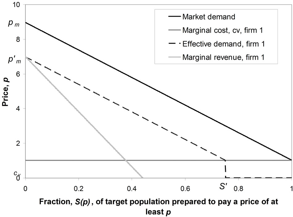
Figure 12. The demand curve of firm 1 in the Cournot model.
tion to supply the whole market by deliberately limiting their maximum feasible output. Under these conditions, Cournot’s model offers a useful insight into oligopoly behaviour, while yielding a clearly defined demand curve of the shape we have considered previously.
Half a century later, Hall and Hitch [7] and Sweezy [8] came up independently with similar specifications for the general form for an oligopolistic demand curve. Sweezy suggested that, in the case of oligopoly, the effective demand curve would be concave, with a kink linking two downwardly inclined lines he drew as essentially straight, but with the second line having a more negative slope. The kinked demand curve may be seen as an asymmetric combination of the Bertrand and Cournot assumptions and suggested that oligopolistic prices would tend to be sticky. This made the construct controversial amongst some economists such as Stigler [9], who considered the rapid adjustment of prices a fundamental economic tenet. The authors give no opinion either way, but include the kinked demand curve for the sake of argument and completeness.
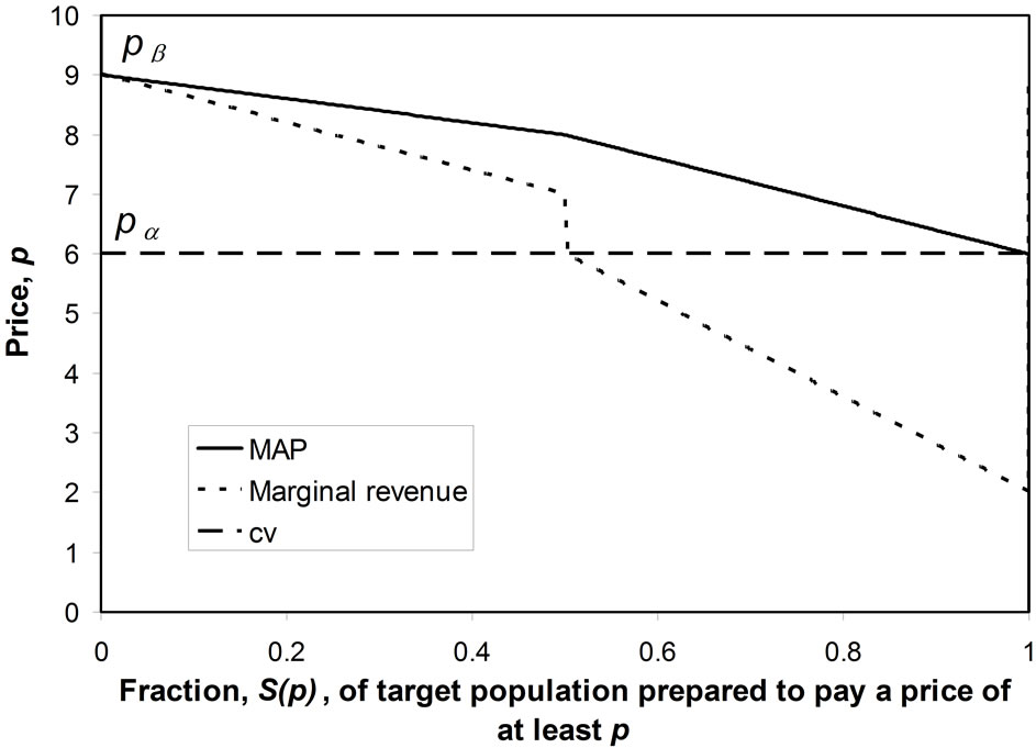
The piecewise linear, kinked demand curve, shown in Figure 13(a), has a corresponding demand density curve that exhibits a step, with the ratio of the probability densities before and after the step being the ratio, r, of the slopes of the demand curve before and after the kink. See Figure 13(b).
Figure 14 shows a contour plot for a constant ratio of the mean price to the optimal price for a kinked demand curve. It is clear that the mean price lies within 10% of the optimal price for a wide range of values of , provided the post-kink slope multiplier, r, is 2 or less. Equally, the mean price will be within 10% of the optimal for a wide range of values of r, provided the ratio of upper and lower prices,
 , is 2 or less. If both
 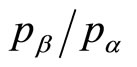 and r are below 2, then the discrepancy between the mean price and the optimal price must be be-
 (a)
(a) (b)
(b)
Figure 13. The kinked demand curve and its corresponding demand density. k, r, pα and pβ are defined in Figure 13(b). (a) Demand curve when: ; (b) Corresponding demand density.
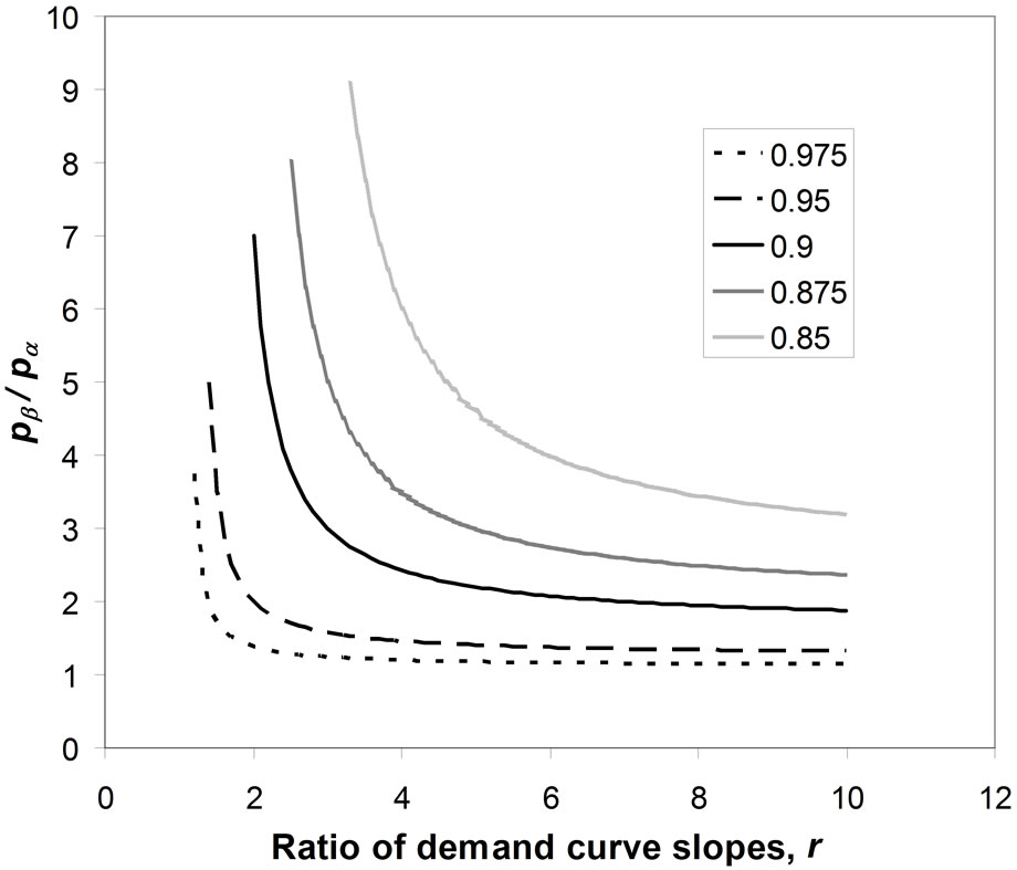
Figure 14. Contour plot of constant ratio of the mean price to the optimal price for kinked demand curve.
low 5%. For the example shown in Figure 13, where  and r = 2, then the mean is just 3.1% below the optimal price.
10.3. Perfect Competition
In the case of perfect competition, the demand curve is horizontal, which implies a single price set by the market, not subject to change by the retailer. The corresponding demand density curve will be an impulse at the market price—a rectangular pulse of unit area with a width approaching zero and a height approaching infinity, a function known to physicists as a Dirac delta function. Self evidently all central measures, such as the mean and median of the distribution and the mean of the matched Rectangular distribution, will converge to a single value under these conditions, which value will also constitute the optimal price.
10.4. Summary of the Results for Situations Other than Monopoly
Demand curves that are continuous and downward sloping will characterize both monopolistic competition and oligopoly in the case where Cournot’s theory gives an adequate characterization. These will imply a demand density, h(p), that will exist over some finite, non-zero range of prices. It will be possible to approximate such a demand density by a Rectangular demand density, the mean of which (the matched Rectangular mean) can be expected to approximate the optimal price reasonably well.
Another possibility has been examined in the case of oligopoly, namely the kinked demand curve. This has been shown to correspond to a stepped demand density curve. It is found that the mean of the kinked probability distribution will be similar to the optimal price for a plausible range of its principal parameters.
In the case of perfect competition, the proposition that the mean and the matched Rectangular mean will approximate the optimal price is satisfied exactly, if trivially: all the central measures converge to the single market price in this case.
Thus the mean of the matched Rectangular demand density can be expected to provide a good approximation to the optimal price in all market situations.
11. Estimating the Optimal Retail Price with Minimum Market Testing
The fact that the matched Rectangular mean gives a good approximation to the optimal price for a near-exhaustive range of demand densities means that a simple method may be advanced to estimate the optimal price. The method is aimed at overcoming the difficulty the retailer may have in providing an accurate estimate of the highest price in the retailer’s mental model, . It is assumed that the retailer will be able to determine his variable cost per item,
  , to good accuracy, thus fixing the lowest MAP of interest,
 .
.
The algorithm is based on the minimum amount of market testing, using just two price levels,  , i = 1, 2, where
 . These will lead to two different numbers,
  , i = 1, 2, of consumers buying the product where:
 (14)
(14)
Meanwhile, from Equation (1) the fraction of the market prepared to pay at least  will be:
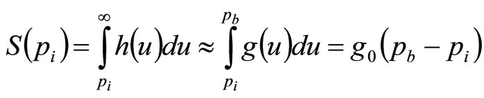 (15)
(15)
where  is the rectangular distribution given in Equation (7), and
 . Hence, combining Equations (14) and (15),
 (16)
(16)
Thus the ratio,  , of the numbers of customers buying at prices,
  and
and , will be:
 (17)
(17)
so that the estimate of the highest price in the retailer’s mental model,  , is then
 (18)
(18)
The estimate of the optimal price is then simply the mean of the Rectangular distribution:
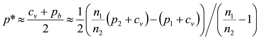 (19)
(19)
This algorithm has been tested against a number of Double Power demand densities, and proved to be highly accurate when the initial price level,  , is already close to the underlying optimum (which should be so even if the retailer had available only the sparse information on price discussed in Section 4), and the price perturbation,
  , is of the order of 10% or less.
Hence, for the demand density shown in Figure 7(a), when the price level is set first at  and second at
 , the algorithm gives an estimated optimal price of 5.35 units, compared with the true optimum calculated for the underlying demand density of 5.34 units.
Meanwhile, for the demand density of Figure 8(b), setting the price levels at  then
then  leads the algorithm to predict an optimal price of 6.16 units, compared with the true optimum calculated for the underlying demand density of 6.17 units.
It may be noted that the extra information coming from the simulated market testing has improved upon the first approximations to the optimal prices coming from the matched Rectangular mean, which were 5.13 units and 6.30 units respectively.
12. Conclusions
A perfect knowledge of the distribution of MAP, or demand density, would enable the retailer to extract the maximum profit, but using market surveys in an effort to obtain such comprehensive and accurate information would be expensive and problematical even if the number of items researched were small. Recognizing the impracticality of repeated market surveys for each and every retail good, the study has tested a near-exhaustive range of possible demand density curves, as embodied in candidate sets 1 and 2. The evidence of the study is that the optimal price may be approximated reasonably well by the mean of the underlying distribution for all the candidate demand densities.
It has been found that all the demand densities considered may be matched well with a Rectangular demand density, which yields an optimum price equal to the mean price. The mean of the matched Rectangular demand density has been found to lie close to the optimum price of the underlying distribution for all the candidate demand densities considered. This is in itself an important result, since the matched Rectangular demand density is likely to correspond to the retailer’s initial mental model of demand density. It suggests that the retailer will be able to make a reasonable initial estimate of the optimal price to charge based on rather sparse price data.
An improved estimate may be found if the retailer is prepared to use the minimum of market testing, using a single perturbation from his initial price. An algorithm has been developed using the assumption that the underlying demand distribution may be approximated well by a Rectangular demand distribution. Worked examples show that the price estimated by the algorithm is an improvement on the mean of the matched Rectangular demand density and is very close to the actual optimal price based on the true, underlying distribution, whatever it is.
The results apply to all the basic forms of interaction between the retailer and his customers, monopoly, monopolistic competition and oligopoly, as well as, in their limiting form, to perfect competition.
13. Acknowledgements
The authors are grateful to Sir John Kingman and Mr Roger Jones for their helpful and useful comments on earlier drafts.
REFERENCES
- R. G. Lipsey and K. A. Chrystal, An Introduction to Positive Economics,” 8th Edition, Oxford University Press, Oxford, 1995.
- D. Begg, S. Fischer and R. Dornbusch, “Economics,” 3rd Edition, McGraw-Hill, London, 1991.
- G. F. Stanlake, “Introductory Economics,” 5th Edition, Longman, Harlow, Essex, 1989.
- Institute of Fiscal Studies (IFS), 2010. http://www.ifs.org.uk/wheredoyoufitin/
- A. A. Cournot, “Recherches sur les Principes Mathématiques de la Richesse,” Chez L. Hachette, Paris, 1838. http://books.google.co.uk/books?id=K2VHAAAAYAAJ&printsec=frontcover&source=gbs_ge_summary_r&cad=0#v=onepage&q&
- J. Bertrand, “Review of ‘Théorie Mathématique de la Richesse Sociale’ and ‘Recherches sur les Principes Mathématiques de la Richesse’,” Journal des Savants, 1883, pp. 499-508.
- R. L. Hall and C. J. Hitch, “Price Theory and Business Behaviour,” Oxford Economic Papers, No. 2, 1939, pp. 12-45.
- P. M. Sweezy, “Demand under Conditions of Oligopoly,” Journal of Political Economy, Vol. 47, No. 4, 1939, pp. 568-573. doi:10.1086/255420
- G. Stigler, “Kinky Oligopoly Demand and Rigid Prices,” Journal of Political Economy, Vol. 55, No. 5, 1947, pp. 432-449. doi:10.1086/256581