Natural Resources
Vol.09 No.12(2018), Article ID:89628,20 pages
10.4236/nr.2018.912028
Development of a Three-Layer Steady State Vertical Dissolved Oxygen Model in Grand Lake, Oklahoma
Josephus F. Borsuah1*, Scott Stoodley1, Daniel Storm1, Andrew Dzialowski1, Andrew Stoddard2
1Oklahoma State University, Stillwater, Oklahoma, USA
2Dynamic Solutions, LLC, Knoxville, Tennessee, USA

Copyright © 2018 by authors and Scientific Research Publishing Inc.
This work is licensed under the Creative Commons Attribution International License (CC BY 4.0).
http://creativecommons.org/licenses/by/4.0/


Received: October 23, 2018; Accepted: December 26, 2018; Published: December 29, 2018
ABSTRACT
Grand Lake O’The Cherokees, the third largest reservoir located in northeastern Oklahoma, provides recreational services, water supply, hydroelectric power, and flood control to residents of Oklahoma and neighboring states. Grand Lake has experienced major problems with eutrophication, harmful algal blooms, and dissolved oxygen (DO) depletion during summer. To better understand the dynamics of DO depletion in the hypolimnion of Grand Lake, a three-layer steady state vertical DO model for summer-stratified conditions was used to investigate dissolved oxygen profiles both above and below the thermocline. The DO model was used to determine the relative effects of atmospheric reaeration and phytoplankton production as a source of DO and phytoplankton respiration, decomposition of organic matter, and nitrification as loss terms for DO. Additionally, the importance of sediment oxygen demand (SOD) for hypolimnetic oxygen depletion was investigated at the sediment water-interface under stratified conditions. Observed water quality data, kinetic coefficients from the literature, and physical, biological, and chemical data collected throughout 2013 and 2015 along the spatial gradient of riverine, transition, lacustrine zones and a site close to the Grand Lake Pensacola Dam were used in the pre-processing calculations to derive estimates of kinetic rates as input parameters to the model. The estimated predictions from the model showed reasonable agreement with the observed vertical profiles of DO. Conclusions from this study indicate that phytoplankton production, high light limitation, and phosphorus were the major terms that controlled DO production in the surface layer, while nitrification and organic carbon decomposition were the major sinks of DO consumption in the bottom layer. Interestingly, SOD did not play a significant role in DO depletion in the water column.
Keywords:
Eutrophication, DO Depletion, Primary Production, Vertical Model, Nutrients, Reservoir, Hypolimnion, Central Plains

1. Introduction
Nutrient Enrichment, Eutrophication and Oxygen Depletion in Lakes and Reservoirs
In the process of retaining minimal level of nutrients in lakes, rivers, and streams to support lakes productivity, the nutrients accumulate overtime causing eutrophication within the water column [1]. By definition, eutrophication in lakes and reservoirs is caused by over enrichment of lakes and reservoirs with high level of nutrients (nitrogen and phosphorus). In most cases, excess levels of nutrients lead to accumulations of high levels of algal biomass including harmful algae blooms that alters the aquatic environment [2]. Some major effects of eutrophication include nuisance levels of algae, taste and odor problems with water supply, occurrence of harmful algae blooms, increased bacterial production, and depletion of DO within the hypolimnion of lakes and reservoirs [3] [4] [5]. In the United States, impairment of approximately 60% of lakes, rivers, and reservoirs is a result of nutrient enrichment and eutrophication [3]. For example, freshwater impairments due to eutrophication have been documented as an important factor affecting the economy of counties, states, and other sectors in United States [6]. As an example, costs related to harmful algae blooms in eutrophic lakes and reservoirs that provide drinking water services and other recreational activities have risen for water treatment costs to over a million United States (US) dollars per algal bloom event, while assessment and monitoring costs in impaired waterbodies have exceeded $50 million US dollars annually [3].
In 2010, 2012, and 2014 the lower segment of Grand Lake was listed in Oklahoma’s Integrated Report of the 303(d) list of impaired waterbodies for the state. The causes of impairment shown on the 303(d) list included low dissolved oxygen (DO) levels. Major contributing factors for low DO were summer stratification and the effects of algal blooms [7]. On July 4, 2011, Grand Lake, the third largest lake in Oklahoma experienced a significant harmful algal bloom of blue-green algae. The Grand River Dam Authority (GRDA) prohibited swimming in the lake and huge tourism-related financial losses were incurred by the regional economy over the July 4th holiday.
Hypolimnetic depletion of DO is a common occurrence in lakes and reservoirs during the summer months in the Central Plains because of seasonal thermal stratification. The formation of a thermocline reduces the resupply of DO from the upper mixed layer to reduce DO levels in the hypolimnion to less than 2 mg/L. Under the Clean Water Act (CWA), water quality management planning efforts by the State of Oklahoma to develop Total Maximum Daily Loads (TMDLs) for lakes and reservoirs are based on models that describe the cause-effect relationships between watershed loading and the seasonal occurrence of hypolimnetic DO depletion.
DO modeling in natural waters has evolved from simple one-dimensional, steady-state “Streeter-Phelps BOD-DO” stream models that accounted for atmospheric reaeration and organic matter mineralization [8] [9] to advanced three-dimensional, time variable biogeochemical models that account for physical transport processes and eutrophication related interactions of nutrients, organic matter, sediment diagenesis, and phytoplankton production with DO [10] and [11] Although advanced models provide the highest resolution to characterize horizontal, temporal, and vertical DO distributions in a waterbody, the level of effort and the field data required to calibrate an advanced lake model requires a commitment of substantial resources and time.
As horizontal gradients of DO in a lake or reservoir are much smaller than vertical gradients, seasonal stratification is a major physical process that controls hypolimnetic DO depletion. One-dimensional (vertical) models, developed to represent horizontally averaged, depth-dependent distributions of DO, can provide insight for assessments of the relative importance of physical and biogeochemical processes that control the formation of seasonal DO profiles in a reservoir or lake. Initial progress for a water quality planning study can be made with a vertical DO model and modest resources to understand the key processes that control hypolimnetic DO depletion in a lake or reservoir.
Models have been developed to represent vertical profiles of DO above and below the thermocline using approaches based on mixed layer box models and continuous diffusive mixing in the water column. Bell [12] developed a time dependent two-layer DO model of Bassenthwaite Lake in England and O’Connor and Mancini [8] developed a steady-state two-layer model of DO in the New York Bight. Steady-state three-layer DO models have been developed for Chesapeake Bay [13] and Tenkiller Ferry Lake [14]. Mixed layer model input parameters were calibrated to account for stratification and components of the DO balance based on kinetic processes and observed data sets. Diffusive mixing models, developed to account for a stack of multiple layers of the water column, have been coupled with physical models of water temperature to represent stratification. Input parameters for DO components have been based on model calibration, kinetic processes, and observed data sets [15] and [16] and coupling of the DO sub-model with physical and biogeochemical models [17].
The objective of this study is to develop a simplified three-layer, steady state vertical DO model for representative station locations in Grand Lake, Oklahoma. Model input parameters developed to represent thickness of the three layers, DO sources from reaeration and phytoplankton production and DO sinks from sediment oxygen demand and DO consumption are derived from observed data and calibration of kinetic coefficients. In addition, derived model input rates and kinetic processes are used to determine the relative importance of DO source sink terms on DO depletion within the hypolimnion of Grand Lake under summer-stratified condition.
2. Materials and Methods
With a drainage area of 10,298 square miles, Grand Lake O’The Cherokees stretches through Delaware, Ottawa, and Mayes counties in the northeast area of Oklahoma. The lake is a multi-use reservoir formed from the construction of the Pensacola dam in 1941. A hydrographic survey by OWRB (2009) showed that the surface area and storage volume of the lake has decreased by about 10% from the 1940 design specifications. The physical characteristics of the lake include surface area of 41,779 acres (16,907 ha), mean depth of 36.3 ft (11.1 m), maximum depth of 133 ft (40.5 m), and cumulative storage volume of the lake of 1,515,415 acre-feet [18] and [19]. The lake provides flood control, hydroelectric power supply, drinking water, recreational activities, fish, and wildlife propagation for the state of Oklahoma. The primary land use is agriculture [20] ; the three major tributaries to the lake are the Neosho River, Elk River, and Spring River as shown in Figure 1 below.

Figure 1. Location map showing three major watersheds and tributaries of Grand Lake [20].
2.1. Description of the Model
VERTDO3 is a steady state, one-dimensional analytical model that describes the effect of stratification, biological, and chemical processes on the vertical distribution of dissolved oxygen in lakes and reservoirs [13]. The model assumes steady state conditions and negligible horizontal gradients of DO. The dominant vertical gradient in the water column is represented with three-layers defined as the epiliminion (euphotic layer), metalimnnion (thermocline layer), and hypolimnion. The model has been used as a simplified approach to provide insight into the key physical, chemical, and biological factors that influence the occurrence of anoxia and hypoxia below the thermocline [14]. The mass balance differential equations, analytical solutions, and model parameters for each of the three mixed layers are given in Appendix A.
2.2. Model Development
Water quality in a lake or reservoir is controlled by watershed and wastewater derived pollutants loads, bathymetry, physical transport processes, biological, and chemical reactions. Mathematical model representations, based on mass balance relationships, have been used to quantify the cause-effect relationships that link external pollutants inputs to the water quality response in a lake or reservoir in time and space. Researchers use water quality models in order to predict and interpret water quality responses using mathematical simulation techniques with numerical formulations that represent the response of the water body to external inputs [21]. In this study, a simplified water quality model of the vertical profile of DO was used to account for source terms of oxygen including: atmospheric reaeration and phytoplankton production, and sink terms of oxygen including: SOD, phytoplankton respiration, organic matter decomposition, and nitrification.
2.3. Sources of Data
Water quality monitoring on Grand Lake (Hydrologic Unit Code HUC_8: 11070206) has been ongoing since June 1986. However, the number of sampling points and sampling sites has varied over the years. Currently, 13 different sampling sites are monitored and data from four of these sites were used in this study. The water quality parameters considered in our study included; surface grab samples at 1-meter depth for dissolved oxygen (DO), water temperature, pH, total nitrogen (TN), total phosphorus (TP), chlorophyll a, nitrate (NO3-), Secchi depth, turbidity (NTU), and conductivity. Subsurface water chemistry data collected within the thermocline and hypolimnion layer at varying depths were also used for developing the model.
The lake was represented by the following four zones: Riverine, Transition, Lacustrine, and Dam as shown in Figure 2. Characterization of the lake as four zones is based on physical transport processes in a reservoir such as Grand Lake. In the upper segment of the reservoir, transport resembles river transport and

Figure 2. Schematic illustration of the four zones in Grand Lake [22].
the Riverine Zone is characterized by faster velocity, shorter residence time, and high concentrations of bioavailable substances, higher turbidity, and greater light extinction compared to downstream portions of the lake. Within the middle area of the reservoir, Transition Zone processes are characterized by horizontal gradients, higher phytoplankton productivity and biomass with lower velocity, lower turbidity, longer residence time, and higher sedimentation out of the water column and greater light penetration. The Transition Zone is typically the most productive area of the reservoir. In the lower segment of the reservoir, transport processes are characterized by horizontal and vertical gradients that resemble transport and mixing in open waters of a lake. The Lacustrine Zone is the portion of the lake closest to the dam and can be characterized with lowest velocity, longest residence time, lower concentrations of nutrients and suspended sediment, greater water transparency, and a deeper euphotic zone than the transition and riverine zones [22].
In this study, the three lake layers were determined based on temperature variation measured at different depths (epiliminion, thermocline, and hypolimnion). The epiliminion and hypolimnion were defined by the change in water temperature characterized by a vertical gradient ≤ 1 C m−1 [23] and the thermocline was defined by visual inspection of the depths showing the maximum temperature gradient within the thermocline. Grand Lake was observed to have strongest stratification during June and July, which caused the lake to become anoxic, especially in the deeper parts of the lake at the site close to the dam. Calibration of the model was performed using observed water column data collected by GRDA in 2013 and 2015. Both physical and chemical data were used in the analysis. Physical data included water temperature, station depth, Secchi depth, solar radiation, and wind speed. Chemical data included Ortho-phosphate, Nitrate-N, Chlorophyll-a, DO, Ammonia-N, total nitrogen, total phosphorus, and total organic carbon.
2.4. Kinetic Coefficients and Processes
Observed water quality data, collected in Grand Lake in 2013 and 2015 at the four selected sampling sites shown in Figure 3, were analyzed to derive estimates

Figure 3. Map of Grand Lake showing transition, lacustrine, and riverine zones with the four selected sampling sites.
of the rate oxygen production in the surface layer and the rate of oxygen consumption within each layer of the lake (epiliminion, thermocline, and hypolimnion). Vertical profile data of DO and water temperature for various sampling dates were used to determine the thickness of each of the three layers for each sampling event. Averages of each water quality (WQ) constituent were based on the thickness or depths of each layer. Averages of observed WQ observations and layer thicknesses were assigned as input variables for the pre-processing calculations to specify kinetic rates as input to the model. The observed water quality data were used with stoichiometric C:N:P Redfield ratios to derive estimates of total organic carbon (TOC) and total nitrogen (TN). Table 1 gives a summary and the ranges of the kinetic coefficients used in the pre-processing calculations to derive rate reaction inputs to the vertical DO model. Solutions for the three-layer model equations are presented in Appendix A of this paper. Process relationships and equations used to derive kinetic rate reaction coefficients from observed data sets and model parameters are presented below for DO consumption and DO production terms.
Equations (1)-(3) were used to calculate the DO consumption terms; nitrification of ammonia (NH4), organic carbon decomposition (TOC), and phytoplankton respiration [21].

Table 1. Summary and ranges of the kinetic coefficients used as input for the pre-processing calculation at selected stations in Grand Lake.
1) Nitrification of ammonia
(1)
where,
NH4 = Ammonia-N concentration as Mg-N/L
Kn(20) = rate reaction for nitrification at 20˚C with units of day−1
Ø = temperature-dependence coefficient for nitrification of Ammonia-N
T = Water temperature consistent with other references to water temperature ˚C
Oxygen: Nitrogen ratio is the oxygen derived from nitrification as mg O2/mg N
2) Organic carbon decomposition
(2)
where,
Kd(20) = reaction rate of labile organic carbon at 20˚C with units of day−1
Ø = temperature dependence coefficient for decomposition
T = water temperature ˚C
3) Phytoplankton respiration
(3)
where,
Chl = Chlorophyll/algal biomass as µg/L
Kr(20) = Phytoplankton respiration rate Kr (20˚C) 1/day
Ø = temperature dependence coefficient for phytoplankton respiration
C/Chl = Carbon: Chlorophyll ratio as µg C/µg Chl
Oxygen: Carbon = Oxygen: Carbon ratio as mg O2/mg C
Equations (4)-(7) were used to calculate DO production terms as a function of water temperature, nutrients limitation, and light limitation [21]
1) Water temperature dependence
(4)
where;
Kg(20) = maximum growth rate of phytoplankton at 20˚C (day−1)
Øg = Temperature coefficient 1.06 for phytoplankton growth
T = Water temperature ˚C
2) Nutrient Limitation Dependence
The dependence of phytoplankton growth on nitrogen and phosphorus were calculated from the half-saturation equations below:
(5)
(6)
(7)
where,
N = dissolved inorganic nitrogen concentration (NH4-N +NO2-N +NO3-N) (µg N/L)
P = dissolved inorganic ortho-phosphate (OPO4-P) concentration (µg P/L)
Kn and Kp = nutrient limitation half saturation constants (as µg/L) for nitrogen and phosphorus
3) Light Dependence
Equations (8)-(11) were used to estimate the daily average light was computed from [21] :
(8)
where,
Ia = Daily average light received as langleys/day
f = Photoperiod as fraction of 24 hr day
ITOT = Total daily solar radiation as langleys/day
fPAR = fraction of measured light that is photosynthetically available radiation
(9)
The terms for α0 and α1 are given by the following:
(10)
(11)
4) The general equation used to estimate oxygen production in the photic zone
(12)
where,
Pr = Carbon fixation rate (g C m2-day−1)
∆H = Thickness of the euphotic layer (meters)
Pa = Oxygen production (mg/L-day)
2.5. Summary of Model Input Data
Observed water chemistry and physical data obtained from Grand Lake and kinetic coefficients were used as input data to the pre-processing calculation to derive estimates of model input parameters for the vertical DO model. The ranges of model input data obtained from pre-processing calculations are summarized in Table 2.
2.6. Sensitivity Analysis
Sensitivity analyses were performed on a data set collected at one station located in the lacustrine zone (Tree Site) on July 17, 2013. The SOD and vertical mixing coefficient (E2) were the two variables used for the sensitivity analyses. Different values were tested, ranging from low to high values for both SOD and the vertical
Table 2. Summary and ranges of model input data to the vertical DO model.
mixing rate (E2), to observe the possible effects that may occur within each of three layers of the lake when changes in both the vertical mixing and SOD values are evaluated.
3. Results and Discussion
In the development of the three-layer steady state vertical DO model for Grand Lake, observed water quality data were used to calculate the Trophic State Index (TSI) [24] for Grand Lake to help us understand trophic state condition of the lake within the riverine, transition, lacustrine zones, and the site close to the dam. Table 3 and Table 4 summarize the observed data used to determine the TSI lake classification as mesotrophic, eutrophic, and hypereutrophic.
In 2013, the TSI results show that Grand Lake was eutrophic in all the zones except for the riverine zone which was classified as hypereutrophic. On the other hand, the TSI results for 2015 indicate that Grand Lake was hypereutrophic in the riverine and transition zone, while the lacustrine zone and the site close to the dam were classified as eutrophic. Based on the results obtained from the TSI analysis for both 2013 and 2015, Grand Lake can be characterized as a reservoir with high productivity for algae.
4. Model Calibration and Sensitivity Results
The plots in Figure 4 illustrate typical water temperature profiles (Figure 4(a) and Figure 4(c)) and the results of DO model simulations (Figure 4(b) and Figure 4(d)) for 2013 and 2015 survey dates. Water depth is plotted on the horizontal axis of the vertical profiles. The vertical dotted and solid lines in each
Table 3. Means and ranges of Trophic State Index (TSI) for chlorophyll-a, Secchi depth, and total phosphorus (0 - 1 m depth samples) for 2013 Grand Lake data set.
Table 4. Means and ranges of Trophic State Index (TSI) for chlorophyll-a, Secchi depth, and total phosphorus (0 - 1 m depth samples) for 2015 Grand Lake data set.

Figure 4. Water temperature profile and DO model simulation results for Tree station for July 17, 2013 and July 29, 2015 survey dates.
plot mark the breaks in water temperature used to determine depths and thickness of each layer. As can be seen in Figure 4(b) and Figure 4(d), the DO model shows very good agreement with the observed profile data for DO.
The plots in Figure 5 illustrate a water temperature profiles and results of DO model simulations for the P-dam station in Grand Lake. Figure 5(a) and Figure 5(c) water temperature profiles indicate significant stratification conditions in Grand Lake at the dam during summer of 2013 and 2015 respectively. The vertical dotted and solid lines in each plot mark the breaks in water temperature used to determine depths and thickness of each layer. Figure 5(b) and Figure 5(d) show a comparison of the vertical distribution of modeled DO to the observed DO data collected at P-dam Station on Grand Lake for the 2013 and 2015 survey dates. The DO model predictions indicate reasonable agreement with the observations. The exception is shown in Figure 5(b) for the July 2015 survey where the surface results of the model did not match the observed higher levels of DO. This discrepancy in the model prediction for the surface was due to the following reasons: 1). higher light available at the surface of the photic zone, 2) supersaturated conditions for DO of 140% obtained on that survey date indicate very high rates of primary production in the 0 - 2 m of the surface layer that the depth-averaged model over the euphotic zone layer was unable to match.
The graphs in Figure 6(a) and Figure 6(b) illustrate the results of the sensitivity analysis using SOD and the vertical mixing rate as the variables tested to

Figure 5. Water temperature profile and model simulation results for P-dam station for July 17, 2013 and July 29, 2015 survey dates.
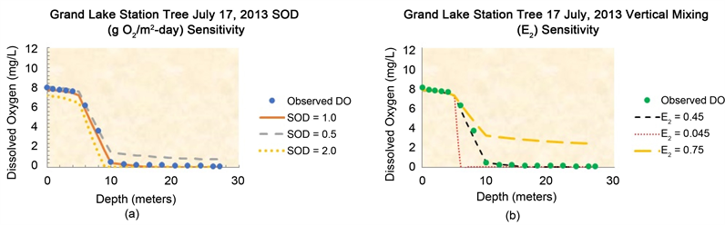
Figure 6. Sensitivity analyses simulation results performed on data obtained at Tree Station on July 17, 2013 survey date.
observe the effects on the model results for Tree Station survey date of July 17, 2013. In Figure 6(a) the circular blue marks are the observed dissolved oxygen, the red line is the base value of SOD = 1.0 g O2/m2-day, the green line is the low value of SOD (0.5 g O2/m2-day) and the purple line is the high value of SOD 2.0 g O2/m2-day). From the graph, the SOD of 1.0 g O2/m2-day shows good agreement with the observed DO throughout the three layers of the water column. The sensitivity tests of the model using the lower (0.5 g O2/m2-day) and higher (2.0 g O2/m2-day) SOD rates showed that neither the low or high SOD rates achieved good agreement with the observed DO. The sensitivity results demonstrate that SOD has an effect on the oxygen profile in all three layers.
In addition to the sensitivity analysis runs using low and high values of SOD (Figure 6(a)), the effect of low and high values of the vertical mixing coefficient (E2) were also tested using parameter values ranging from E2 = 0.045 cm2/sec (low), 0.45 cm2/sec (calibration baseline) to 0.75 cm2/sec (high) respectively. The dramatic effect of the low and high values for the sensitivity analysis of vertical mixing clearly show that the modeled oxygen results for the thermocline layer and the hypolimnion layer are extremely sensitive to the vertical mixing rate assigned for model input. Vertical mixing rates used for development of the vertical DO profile model (see Table 2) were determined by calibration to the observed DO profiles for each station and survey date.
5. Conclusions
A three-layer steady-state model of the vertical structure of DO in a stratified lake has been successfully developed based on observed water chemistry data, physical data such as water depth, water temperature, and kinetic coefficients used to derive input data to the vertical dissolved oxygen model. The model was developed using water quality data collected during the summer months of 2013 and 2015 for stations within the characteristic riverine, transition, lacustrine zones and at the dam in Grand Lake. Application of the model to a set of water quality data obtained for 2013 and 2015 gives an understanding of reservoir eutrophication processes and how physical, chemical and biological processes are connected to DO production and DO consumption in the epiliminion, thermocline, and hypolimnion layers of the lake.
Results obtained from the model simulations at each station and zone give reasonable agreement between the predicted versus observed dissolved oxygen profiles within the water column. Based on the pre-processing analysis used to derive rate estimates for model input, the vertical DO model successfully accounted for both oxygen production terms and oxygen consumption terms. Based on the percentage analysis for each source and sink term, the pre-processing analysis clearly identified the relative importance of each component term for oxygen production and oxygen consumption.
In summary, the relative effects on oxygen production in the photic zone were based on phytoplankton biomass, high light limitation, and nutrient limitation. The relative effects on oxygen consumption were based on the phytoplankton biomass and the levels of organic matter and ammonia in the water column. In a study of Lake Erie, Clevinger [25] found that SOD contributed 19.2 percent to the total oxygen demand in the hypolimnion, while nitrification accounted for 32.6 percent in the hypolimnion and 28 percent of oxygen demand in the epiliminion layer. In contrast to other studies [26] where sediment oxygen demand accounted for a large component of hypolimnetic oxygen demand, Clevinger’s results from Lake Erie are consistent with the results derived from this analysis of the contributions of nitrification and sediment oxygen demand to oxygen consumption in Grand Lake. Key findings from this study show that high light limitation at the surface layer, phytoplankton growth rate, and phosphorus were the most critical factors for oxygen production within the epiliminion layer while nitrogen availability was the least critical factor. Phosphorus was the limiting factor to phytoplankton production in most cases, except for the P-dam site on July 17, 2013 where it was found that nitrogen was the limiting factor for phytoplankton production due to supersaturation conditions of 140 percent at the 0 - 2 m depth and high light limitation observed at the surface.
Analysis of sink terms for oxygen (phytoplankton respiration, nitrification, organic carbon decomposition, and sediment oxygen demand) showed that the most critical factor for oxygen consumption within the entire water column was nitrification and the least critical factor was sediment oxygen demand. The effect of stratification on the oxygen profile was demonstrated with the sensitivity analyses simulation results for the vertical mixing rate. The analysis clearly showed that a smaller mixing coefficient will result in stronger stratification, while a larger mixing coefficient will result in weaker stratification. The model proved to be very useful to provide insight into the relative contributions of the different physical and kinetic processes for formation of the oxygen profile in a stratified lake. The model was able to quantify the relative importance of the different source and sink terms on the seasonal occurrence of hypoxia and anoxia in the hypolimnion.
Acknowledgements
First of all, I thank God for this great opportunity. This study was funded by theEnvironmental Science Graduate Program at Oklahoma State University. The authors ofthis work are grateful for the opportunity and part of it goes to Grand River DamAuthority (GRDA) management for providing data for this work. I would like to thank my advisor Dr. Scott Stoodley, and committee members Dr. Daniel E. Storm, Dr. Andrew R. Dzialowski, and Dr. Andrew Stoddard for their meaningful contributions throughout this study. Finally, I dedicate this work to Borsuah, Mansaray, and Kamara family.
Conflicts of Interest
The authors declare no conflicts of interest regarding the publication of this paper.
Cite this paper
Borsuah, J.F., Stoodley, S., Storm, D., Dzialowski, A. and Stoddard, A. (2018) Development of a Three-Layer Steady State Vertical Dissolved Oxygen Model in Grand Lake, Oklahoma. Natural Resources, 9, 448-467. https://doi.org/10.4236/nr.2018.912028
References
- 1. Correll, D.L. (1999) Phosphorus: A Rate Limiting Nutrient in Surface Waters. Poultry Science, 78, 674-682. https://doi.org/10.1093/ps/78.5.674
- 2. Elser, J.J., Sterner, R.W., Galford, A.E., et al. (2000) Pelagic C:N:P Stoichiometry in a Eutrophied Lake: Response to a Whole-Lake Food-Web Manipulation. Ecosystems, 3, 293-307. https://doi.org/10.1007/s100210000027
- 3. Smith, V.H. (2003) Eutrophication of Freshwater and Coastal Marine Ecosystems a Global Problem. Environmental Science and Pollution Research, 10, 126-139. https://doi.org/10.1065/espr2002.12.142
- 4. David, W.S., Hecky, R.E., Findlay, D.L., et al. (2008) Eutrophication of Lakes Cannot Be Controlled by Reducing Nitrogen Input: Results of a 37-Year Whole-Ecosystem Experiment. Proceedings of the National Academy of Science, 105, 11254-11258. https://doi.org/10.1073/pnas.0805108105
- 5. Carter, L.D. and Dzialowski, A.R. (2012) Predicting Sediment Phosphorus Release Rates Using Land Use and Water-Quality Data. Freshwater Science, 31, 1214-1222. https://doi.org/10.1899/11-177.1
- 6. Dodds, W.K., Bouska, W.W., Eitzmann, J.L., et al. (2009) Eutrophication of U.S. Freshwaters: Analysis of Potential Economic Damages. Environmental Science and Technology, 43, 12-19. https://doi.org/10.1021/es801217q
- 7. ODEQ (2014) Oklahoma 303(d) List of Impaired Waters, Appendix C. Oklahoma Dept. Environmental Quality, Oklahoma City.
- 8. O’Connor, D.J. and Mancini, J.L. (1979) The Carbon-Oxygen Distribution in New York Bight, Phase I Steady State. Manhattan College, Environmental Engineering & Science Program, Riverdale, Prepared for MESA New York Bight Project, NOAA Marine Ecosystem Analysis, Stony Brook.
- 9. Streeter, H.W. and Phelps, E.B. (1925) A Study of the Pollution and Natural Purification of the Ohio River, U.S. Public Health Service Bulletin, No. 146, 1-75.
- 10. Ji, Z.-G. (2017) Hydrodynamics and Water Quality Modeling Rivers, Lakes, and Estuaries. 2nd Edition, John Wiley & Sons, Inc., Hoboken. https://doi.org/10.1002/9781119371946
- 11. Pena, M.A., Katsev, S., Oguz, T. and Gilbert, D. (2010) Modeling Dissolved Oxygen Dynamics and Hypoxia. Biogeosciences, 7, 913-957.
- 12. Bell, V.A., George, D.G., Moore, R.J. and Parker, J. (2006) Using a 1-D Mixing Model to Simulate the Vertical Flux of Heat and Oxygen in a Lake Subject to Episodic Mixing. Ecological Modelling, 190, 41-54. https://doi.org/10.1016/j.ecolmodel.2005.02.025
- 13. Hydro Qual, Inc. (1986) Development of a Hydrodynamic and Water Quality Model of Chesapeake Bay. Prepared by Hydro Qual, Inc. for Battelle Columbus Laboratories and EPA, Chesapeake Bay Program, Annapolis.
- 14. DSLLC (2005) EFDC Support Services to Oklahoma DEQ to Support Development of Total Maximum Daily Loads (TMDL) for Tenkiller Ferry Lake, Task 4B Technical Memorandum: An Analysis of the Vertical Structure of Dissolved Oxygen in a Stratified Lake. Prepared by Dynamic Solutions, LLC, Knoxville, TN for Oklahoma Dept. of Environmental Quality, Oklahoma City.
- 15. Rucinski, D.K., Beletsky, D., DePinto, J.V., Schwab, D.J. and Scavia, D. (2010) A Simple 1-Dimensional, Climate Based Dissolved Oxygen Model for the Central Basin of Lake Erie. Journal of Great Lakes Research, 36, 465-476. https://doi.org/10.1016/j.jglr.2010.06.002
- 16. Stefan, H.G., Wright, D., Easton, J.G. and McCormick, J.H. (1995) Simulation of Dissolved Oxygen Profiles in a Transparent, Dimictic Lake. Limnology and Oceanography, 40, 105-118. https://doi.org/10.4319/lo.1995.40.1.0105
- 17. Soetaert, K. and Middelburg, J.J. (2009) Modeling Eutrophication and Oliogotrophication of Shallow-Water Marine Systems: The Importance of Sediments under Stratified and Well-Mixed Conditions. Hydrobiologia, 629, 239-254. https://doi.org/10.1007/s10750-009-9777-x
- 18. Nikolai, S.J. and Dzialowski, A.R. (2014) Effects of Internal Phosphorus Loading on Nutrient Limitation in a Eutrophic Reservoir. Limnologica-Ecology and Management of Inland Waters, 49, 33-41. https://doi.org/10.1016/j.limno.2014.08.005
- 19. OWRB (2009) Hydrographic Survey of Grand Lake. Oklahoma Water Resources Board, Oklahoma City.
- 20. Grand Lake O’ the Cherokees Watershed Alliance Foundation, Inc. (2008) Grand Lake Watershed Plan for Improving Water Quality throughout the Grand Lake.
- 21. Chapra, S.C. (1997) Surface Water Quality Modeling. McGraw Hill Publishing, New York, 844 p.
- 22. Green, W.R., Robertson, D.M. and Wilde, F.D. (2015) Chapter A10. Lakes and Reservoirs: Guidelines for Study Design and Sampling. No. 9-A10, US Geological Survey.
- 23. Nikolai, S.J. (2012) Eutrophication in Grand Lake, Oklahoma: Nutrient Limitation and the Effect of Internal Phosphorus Loading. Oklahoma State University, Stillwater.
- 24. Carlson, R.E. (1977) A Trophic State Index for Lakes. Limnology & Oceanography, 22, 361-369. https://doi.org/10.4319/lo.1977.22.2.0361
- 25. Clevinger, C.C. (2013) Nitrifiers and Their Contribution to Oxygen Consumption in Lake Erie. Doctoral Dissertation, Kent State University, Kent.
- 26. Pace, M.L. and Prairie, Y.T. (2005) Respiration in Lakes. In: del Giorgio, P.A. and Williams, P.J.B., Eds., Respiration in Aquatic Ecosystems, Oxford University Press, New York, 103-121. https://doi.org/10.1093/acprof:oso/9780198527084.003.0007
- 27. Diaz, R.J. and Rosenberg, R. (2008) Spreading Dead Zones and Consequences for Marine Ecosystems. Science, 321, 926-929. https://doi.org/10.1126/science.1156401
Appendix A: Three Layer Steady State Model for Dissolved Oxygen in a Stratified Lake or Reservoir
A one-dimensional model has been developed to simulate the vertical profile of dissolved oxygen (DO) under summer stratified conditions. The model, based on a conceptual representation of the vertical structure of water temperature in a lake or reservoir as three mixed layers in a stratified water column, represents the epiliminion, metalimnnion, and hypolimnion as shown in Figure A1 of Appendix-A. The model, based on mass balance principles, is developed from analytical solutions of the three layer set of coupled differential equations presented in [13]. Kinetic relationships used to derive model input values from observed data for model parameters listed in this appendix are presented in Table 1 of this paper. Model parameter values used to develop the model are summarized in Table 2.
The differential equation for the surface euphotic zone layer (n = 1) is given by;
the equation for the surface layer, D is the oxygen deficit; E1 is the rate of vertical mixing within the surface layer; and R1 is water column consumption of oxygen from algal respiration, nitrification and decomposition of detrital organic carbon; whereas Pa is the depth integrated algal photosynthetic production of oxygen within the euphotic zone [21].
The differential equation for the thermocline layer (n = 2) and the hypolimnion layer (n = 3) is depicted by;

Figure A1. Water temperature-depth profile showing conceptual representation of three mixed layers in a stratified lake or reservoir.
The differential equations for each layer were integrated to give solutions for each layer (n = 1, n = 2, and n = 3). The water column oxygen consumption computed for each layer from nitrification, algal biomass respiration and detrital organic carbon decomposition is depth-integrated over the entire water column to yield a depth-averaged rate of oxygen consumption applied as a constant (R) to each layer. The surface layer depth-averaged photosynthetic oxygen production rate (Pa) is computed from chlorophyll-a (algal biomass), carbon: chlorophyll and oxygen: carbon stoichiometric ratios for algae, and the algal growth rate computed as a function of water clarity, light availability, ambient nutrient concentrations and water temperature [21].
At the air-water boundary of the surface layer (n = 1) the dissolved oxygen deficit is computed from:
where,
Do = is the oxygen deficit (mg/L)
S = Sediment oxygen demand (g O2 m−2 day-1)
R = Depth averaged water column oxygen consumption (g O2/m3-day)
Pa = Euphotic zone algal oxygen production (g O2/m3-day)
H = Water column depth t the sediment bed-water interface (m)
H1 = Depth at the bottom of the surface euphotic layer (m)
Systematic representation of oxygen deficit in the surface layer (n = 1) was computed from:
Definition of terms and units for surface layer (n = 1) solutions are:
D1(z) = dissolved oxygen deficit at depth, z with the layer (mg/L)
Z = depth in layer (Z = 0 is air-water interface) (m)
S = sediment oxygen demand (g O2/m2-day)
R = depth averaged water column oxygen consumption (g O2/m3-day)
Pa = euphotic zone algal oxygen production (g O2/m3-day)
H = depth at sediment bed-water interface (m)
H1 = depth of the surface layer (n = 1) at interface with thermocline layer (n = 2) (m)
KL = air-water transfer coefficient for oxygen (m/day)
E1 = vertical mixing rate for surface layer (n = 1) (m2/day)
The oxygen deficit Dn(z) for each sub-surface layer (n = 2 and n = 3) is computed from:
(A1)
where,
Dn(z) = Oxygen deficit at depth, z within layer n = 2 and n = 3 (mg/L)
Z = depth in layer n = 2 and n = 3 (Z = 0 is air-water interface; Z = H is bottom depth (m)
H1 = depth of euphotic zone layer (n = 1) at interface with the thermocline layer (n = 2) (m)
H2 = depth of thermocline layer (n = 2) at interface with hypolimnion layer (n = 3) (m)
H3 = depth of hypolimnion layer (n = 3) at interface with sediment bed (n = 3) (m)
H = depth at sediment bed-water interface (i.e., bottom depth) (m)
E2 = vertical mixing rate for thermocline layer (n = 2) (m2/day)
E3 = vertical mixing rate for hypolimnion layer (n = 3) (m2/day)