Open Journal of Civil Engineering
Vol. 2 No. 1 (2012) , Article ID: 17817 , 6 pages DOI:10.4236/ojce.2012.21005
Slope Stability Evaluations by Limit Equilibrium and Finite Element Methods Applied to a Railway in the Moroccan Rif
3GIE Laboratory, Mohammadia Engineering School, Mohammed V-Agdal University, Rabat, Morocco
Email: baba.khadija@gmail.com
Received December 2, 2011; revised January 4, 2012; accepted January 17, 2012
Keywords: Conventional Methods; Finite Elements; Safety Factor; Slopes Stability
ABSTRACT
Since 1930, the analysis of slope stability is done according to the limit equilibrium approach. Several methods were developed of which certain remain applicable because of their simplicity. However, major disadvantages of these methods are (1) they do not take into account the soil behavior and (2) the complex cases cannot be studied with precision. The use of the finite elements in calculations of stability has to overcome the weakness of the traditional methods. An analysis of stability was applied to a slope, of complex geometry, composed of alternating sandstone and marls using finite elements and limit equilibrium methods. The calculation of the safety factors did not note any significant difference between the two approaches. Various calculations carried out illustrate perfectly benefits that can be gained from modeling the behavior by the finite elements method. In the finite elements analysis, the shape of deformations localization in the slope is nearly circular and confirms the shape of the failure line which constitutes the basic assumption of the analytical methods. The integration of the constitutive laws of soils and the use of field’s results tests in finite elements models predict the failure mode, to better approach the real behavior of slope soil formations and to optimize its reinforcement.
1. Introduction
The slope stability analysis is performed with the limit equilibrium method based on assumptions about the sliding surface shape. These methods remain popular because of their simplicity and the reduced number of parameters they require, which are slope geometry, topography, geology, static and dynamic loads, geotechnical parameters and hydrogeologic conditions. However they do not take into account the ground behavior and the safety factors are supposed to be constant along the failure surface.
With continuous improvement of the computer performance, the use of the finite elements in calculations of stability has been developed. These methods have several advantages: to model slopes with a degree of very high realism (complex geometry, sequences of loading, presence of material for reinforcement, action of water, laws for complexes soil behavior…) and to better visualize the deformations in soils in place. The application of these various methods on a concrete case permits more than their comparison to highlight all previously mentioned elements. Various calculations carried out illustrate perfectly benefits that can be gained from modeling the behavior by the finite elements method.
2. Methods of Slope Stability Analysis
2.1. Limit Equilibrium Methods
Limit equilibrium methods are still currently most used for slopes stability studies. These methods consist in cutting the slope into fine slices so that their base can be comparable with a straight line then to write the equilibrium equations (equilibrium of the forces and/or moments). According to the assumptions made on the efforts between the slices and the equilibrium equations considered, many alternatives were proposed (Table 1). They give in most cases rather close results. The differences between the values of the safety factor obtained with the various methods are generally lower than 6% [1].
The traditional methods of slices used are those of Fellenius [2] and Bishop [3]. On Figure 1 is represented the cutting of a portion of slope potentially in rupture. The equilibrium of slice i on the horizontal is written:

The forces applied on the ith slice are defined in Figure 1. Hi and Hi+1 are horizontal inter-slice forces. Vi and Vi+1 are vertical inter-slice forces.

Table 1. The main limit equilibrium methods [4].

Figure 1. Circular failure surface and forces acting on a single slice according to Bishop and Fellenius methods [2,3].
Wi is the weight of ith slice. Ni and Ti are resultant of the normal and tangential forces acting on the ith slice base of length li and inclination αi with respect to the horizontal (Figure 1).
The equilibrium of slice i on the vertical is written:
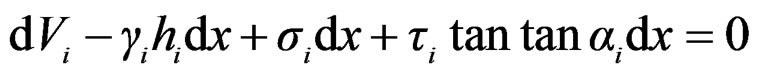
where γi is the unit weight of slice i.
In the method of Fellenius [2], we make the assumption that dHi and dVi are nil, which implies that the normal stresses are estimated by:

By using the total definition of the safety factor, we obtain the equation:

In Bishop’s method of [3], we make the assumption that dVi = 0. Thus, by considering the total definition of the safety factor, we obtain: FBish = F (FBish).
The safety factor is given by using an iterative procedure (see the equation below).
The general procedure in all these methods can be summarized as follows:
• Assumption of the existence of at least one slip surface;
• Static analysis of normal and tangential stresses on the slip surfaces;
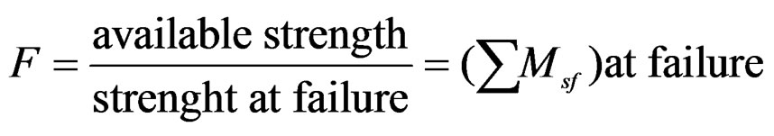
• Calculation of the safety factor F, defined like the ratio of the shear strength on effective shear stress along the failure surface considered;
• Determination of the critical failure surface with safety factor F minimum, among the whole analyzed surfaces.
|

2.2. Finite Element Methods
The various limit equilibrium methods are based on the arbitrary choosing a series of slip surfaces and of defining that which gives the minimal value of the safety factor. Nowadays, we attend an intensive use of numerical analysis methods giving access to the constraints and deformations within the formations constituting the subsoil. For that purpose, it is necessary to know the behaveior law of the considered formations; then, the volume of ground is divided into simple geometric elements, each element being subjected to the action of the close elements.
The calculation will consist in determining stress fields and displacements compatible with the mechanic equations and the behavior law adopted.
Many works were done in the finite elements field and we could cite works of ZIENKIEWICZ [5] or DHATT [6].
The finite element method makes it possible to calculate stresses and deformations state in a rock mass, subjected to its self weight with the assumption of the behavior law adopted. In our calculations, a model with internal friction without work hardening (perfect elastoplastic Model: Mohr-Coulomb) is used, which corresponds to the basic assumptions of the analytical methods.
In our work, we will use the method of reduction of soil resistance properties, known as the “c-φ reduction” method. Many researchers used this method; we can quote works of SAN and MATSUI [7], UGAI [8], etc.
The c-φ method is based on the reduction of the shear strength (c) and the tangent of the friction angle (tanφ) of the soil. The parameters are reduced in steps until the soil mass fails. Plaxis uses a factor to relate the reduction in the parameters during the calculation at any stage with the input parameters according to the following equation:
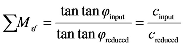
where Msf is the reduction factor at any stage during calculations, tanφinput and cinput are the input parameters of the soil, tanφreduced and creduced are the reduced parameters calculated during the analysis [9].
The characteristics of the interfaces, if there is, are reduced in same time. On the other hand, the characteristics of the elements of structure like the plates and the anchoring are not influenced by Phi-C reduction. The total multiplier SMsf is used to define the value of the soil strength parameters at a given stage in the analysis.
At the failure stage of the slope, the total safety factor is given as follows:
3. Case Study: Railway Slope
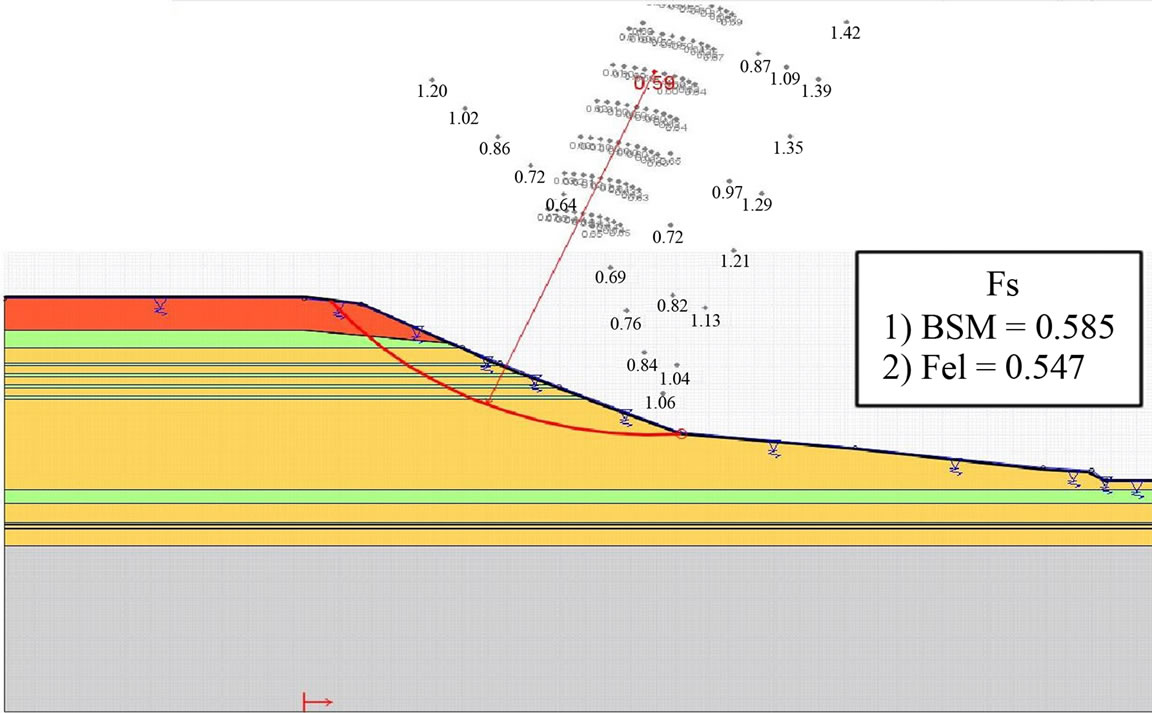
The case study relates to a railway slope in Moroccan Prérif, between Tangier city and Tangier-Med port. The geological formations are consisted of sandstone and marls alternations (Figure 2). The important rains caused a landslide on a ravine which damaged locally the railway.
Calculations are then carried out on the profiles of ground considered to be representative. The geometrical model is on Figure 3. The mechanical characteristics obtained from the laboratory and field tests are represented in Table 2.
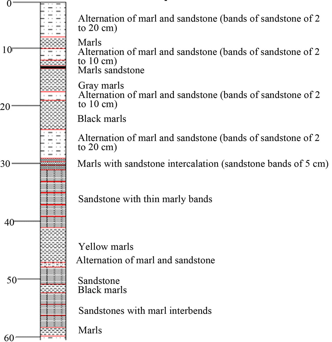
Figure 2. Stratigraphic column of sedimentary formations constituting the embankment.

Figure 3. Finite element mesh of slope profile.
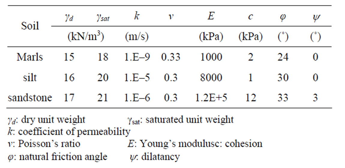
Table 2. Geotechnical parameters of soils.
Calculations are carried out under the two following conditions: dry and saturated states using three softwares Plaxis [9], Geoslope [10] and Talren [11] with the longterm characteristics. The two firsts are based on the limit equilibrium methods whereas the last is a finite elements code. For our study we adopted a model of plane deformation with 15 nodes and 1080 elements (Figure 3).
3.1. Dry State
In our study, the c-φ reduction method according to the Mohr Coulomb criterion underestimates the safety factor about 2% from the value obtained by Fellenius’ method the more conservative method and 7% from Bishop’s method (Figure 4 and Table 3).
 (a)
(a)  (b)
(b)  (c)
(c)
Figure 4.Safety factor Fs in dry state: (a) Talren; (b) Geo- slope and (c) Plaxis.

Table 3. Safety factors in the dry state.
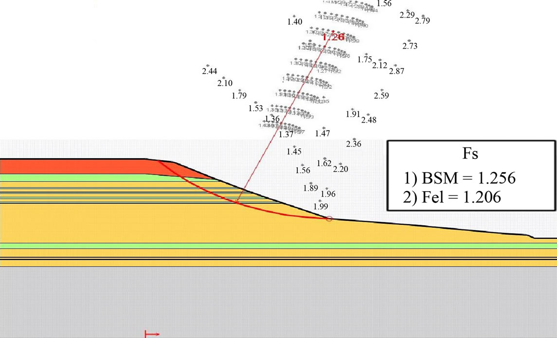
3.2. Saturated State
The preceding calculations were carried out by supposing that the pore water pressures are uniformly null in the slope. The taking into account of the effects of water can be made in various manners according to the calculation method used. The presence of the water table destabilizes the slope and reduces its safety factor (Table 4).
The comparison of the safety factors obtained by the method of c-φ reduction according to the Mohr Coulomb criterion and the analytical methods made it possible to extract the following points (Figure 5 and Table 4):
• The safety factor was over-estimated about 21% compared to Fellenius’ one• The safety factor was over-estimated about 3% compared to Junbo’s one• The safety factor was under-estimated about 3% compared to Bishop’s one• The safety factor was under-estimated about 4% compared to Morgenstern-Price’s one.
3.3. Discussion
The safety factor found using the method of c-φ reduction according to the criterion of Mohr Coulomb remains comparable with those found by the analytical methods in both cases with or without presence of water. The difference noted is the fact that for the analytical methods, safety factors are assumed constants along the failure surface.
Moreover, finite element methods that provide access to stresses and strains within the soil, offer the possibility of a detailed operating calculations as curves: displacements (Figure 6), the evolution of the safety factor according to displacement (Figure 7), the localization of deformations (Figure 8) and plastic zones (Figure 9).
The taking into account of the behavior law in the codes with the finite elements makes it possible to better determine the stress and strain state in various points.
The total displacements figure highlights the limit between the zone where there is no displacement (zero value) and the zones where displacements occur (non null values). We note the circular form of this limit which points out the slip surface adopted by the analytical methods (Figure

Table 4. Safety factors in the saturated state.
 (a)
(a) 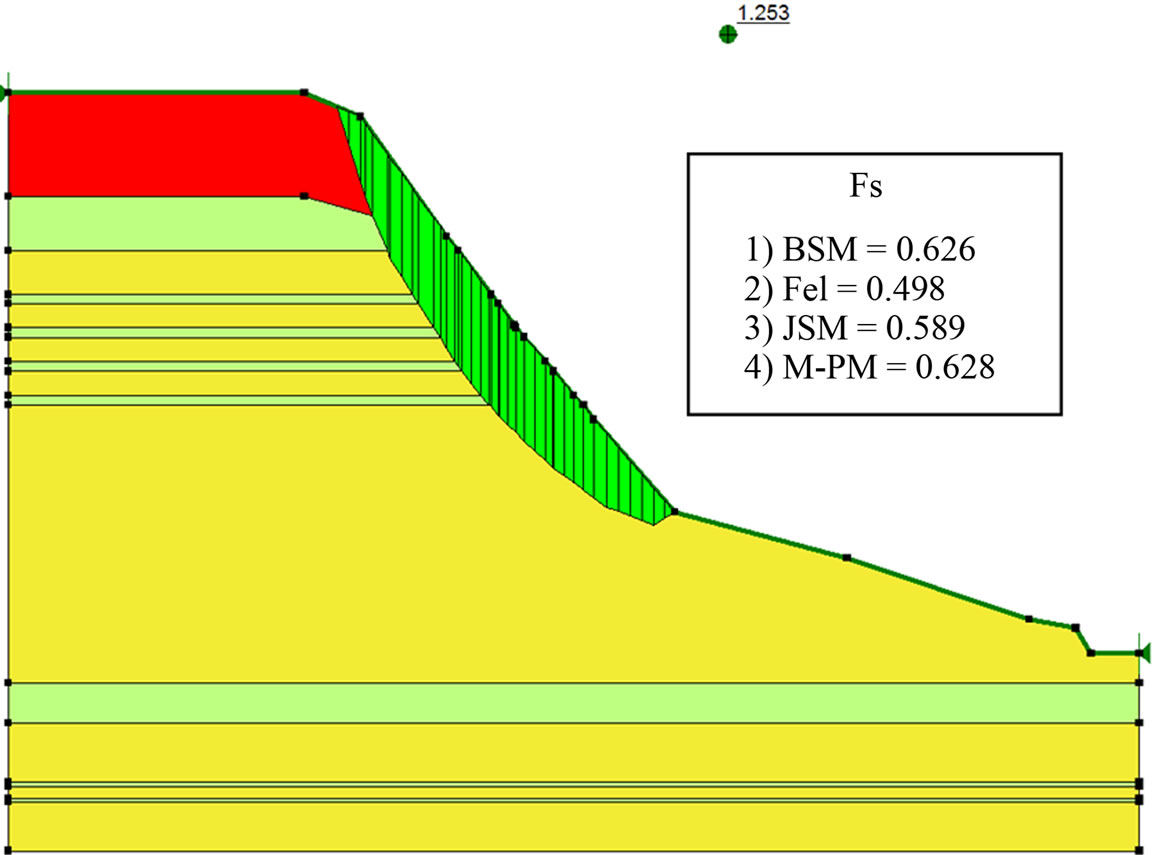 (b)
(b) 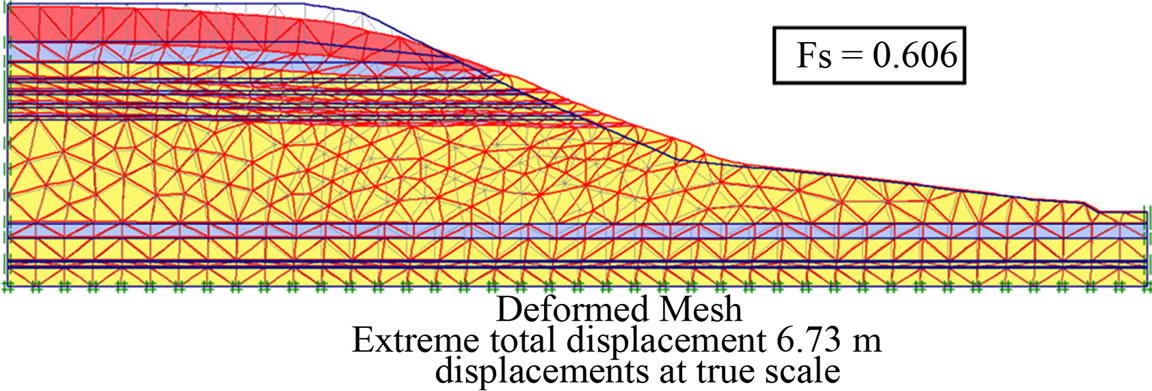 (c)
(c)
Figure 5. Safety factor Fs in saturated state: (a) Talren; (b) Geoslope and (c) Plaxis.
6). These displacements are important at the slope and the highest value is in mid-slope (Figure 7). The horizontal component of displacements exceeds the vertical’s
 (a)
(a) (b)
(b)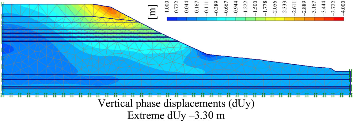 (c)
(c)
Figure 6. Shading of the displacement increments of the embankment in the final stage: (a) Total displacement; (b) Horizontaldisplacement; (c) Vertical displacement.
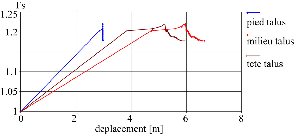
Figure 7. Evolution of safety factor with displacements.

Figure 8. Strains localization.
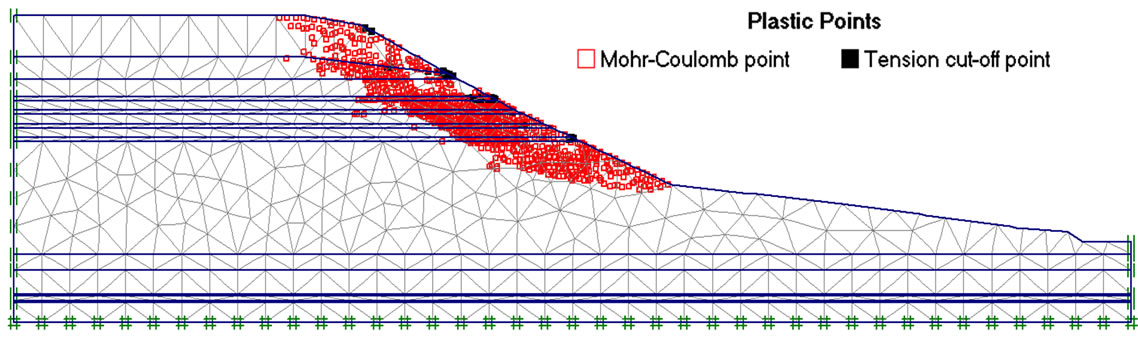
Figure 9. Localization of plastic zones.
(Figures 6(b) and (c)). The rupture curve identification in Plaxis is based on the localization of the deformations on the slope (Figure 8): we once again, find the circular form of slip surfaces. The figure 9 shows the concentration of plastic points inside this same limit.
4. Conclusions
The analysis and design of failing slopes and highways embankment requires an in-depth understanding of the failure mechanism in order to choose the right slope stability analysis method.
The present study made it possible to compare on a real geometrical model the computation results of the safety factor (defining the state of the slope stability compared to the limit equilibrium) by various methods: limit equilibrium and finite elements methods. The behavior law stress-strain which is lacking to the limit equilibrium methods is integrated into the finite elements methods.
The results obtained with slices methods and FEM are similar. However, the results obtained using the finite elements are nearest those obtained by Bishop’s method than Fellenius’ method.
If we compare the sliding surfaces obtained with the slices methods with representations of the total displacement increments obtained with FEM, it is possible to see that the failure mechanism was very well simulated by FEM. In the analyzed case it is possible to see the circular shape of the sliding surfaces in the graphics of the total displacements increments.
The determination of the safety factor is insufficient to identify problems of slope stability, the various calculations performed illustrate perfectly the benefits that can be gained from modeling the behavior by FEM: 1) the calculation of displacements obtained by FEM allows to estimate the actual settlement and optimize ways of reinforcement; 2) the prediction of failure mechanism; 3) the use of the results of field tests to better approximate the real behaviour of structures.
REFERENCES
- J. M. Duncan, “State of the Art: Limit Equilibrium and Finite-Element Analysis of Slopes,” Journal of Geotechnical Engineering, Vol. 122, No. 7, 1996, pp. 577-596. doi:10.1061/(ASCE)0733-9410(1996)122:7(577)
- W. Fellenius, “Erdstatische Berechnungenmit Reibung und Kohasion,” Ernst, Berlin, 1927.
- A. W. Bishop, “The Use of the Slip Circle in the Stability Analysis of Slopes,” Géotechnique, Vol. 5, No. 1, 1955, pp. 7-17. doi:10.1680/geot.1955.5.1.7
- J. M. Duncan, A. L. Buchignani and M. De Wet, “An Engineering Manual for Slope Stability Studies,” Virginia Polytechnic Institute, Blacksburg, 1987.
- O. C. Zienkiewicz and R. L. Taylor, “The Finite Element Method Solid Mechanics,” Butterworth-Heinemann, Oxford, Vol. 2, 2000, p. 459.
- G. Dhatt and G. Touzot, “Une Présentation de la Méthode des Eléments Finis,” Hermes Science Publications, Paris, 1981, p. 543.
- K. C. San and T. Matsui, “Application of Finite Element Method System to Reinforced Soil,” Proceeding International Symposium on Earth Reinforcement Practice, Kyusu, 11 November 1992, pp. 403-408.
- K. Ugai, “Availability of Shear Strength Reduction Method in Stability Analysis,” Tsuchi-to-Kiso, Vol. 38, No. 1, 1990, pp. 67-72.
- PLAXIS, “Finite Element Code for Soil and Rock Analysis,” Brinkgreve, et al., Ed., PLAXIS-2D Version 8, Reference Manual, DUT, the Netherlands, 2004. www.plaxis.nl
- SLOPE/W, “Stability Analysis,” Users Guide Version 5, GeoSlope Office, Canada, 2002. www.geoslope.com
- Talren 4, “Logiciel Pour L’analyse de la Stabilité des Structures Géotechniques,” User Guide Terrasol, Montreuil, 2004.