Journal of Applied Mathematics and Physics
Vol.2 No.7(2014), Article
ID:46806,10
pages
DOI:10.4236/jamp.2014.27059
Determination of Flow Structure in a Gold Leaching Tank by CFD Simulation
C. P. K. Dagadu1*, Z. Stegowski2, L. Furman2, E. H. K. Akaho1, K. A. Danso1
1Ghana Atomic Energy Commission, Legon, Accra, Ghana
2Faculty of Physics and Applied Computer Science, AGH-UST, Krakow, Poland
Email: *dagadukofi@yahoo.co.uk
Copyright © 2014 by authors and Scientific Research Publishing Inc.
This work is licensed under the Creative Commons Attribution International License (CC BY).
http://creativecommons.org/licenses/by/4.0/


Received 14 January 2014; revised 14 February 2014; accepted 22 February 2014
ABSTRACT
Experimental residence time distribution (RTD) measurement and computational fluid dynamics (CFD) simulation are the best methods to study the hydrodynamics of process flow systems. However, CFD approach leads to better understanding of the flow structure and extent of mixing in stirred tanks. In the present study, CFD models were used to simulate the flow in an industrial gold leaching tank. The objective of the investigation was to characterize the flowfield generated within the tank after process intensification. The flow was simulated using an Eulerian-Eulerian multi-fluid model where the RANS standard 𝒌-ε mixture model and a multiple reference frame approach were used to model turbulence and impeller rotation respectively. The simulated flowfield was found to be in agreement with the flow pattern of pitched blade axial-flow impellers that was used for mixing. The leaching tank exhibited good “off-bottom suspension” which reveals minimum deposition of gold ore particles on the bottom of the leaching tanks. Simulation results were consistent with experimental results obtained from a radioactive tracer investigation. CFD approach gave a better description of the flow structure and extent of mixing in a leaching tank. Hence it could be a preferred approach for flow system analysis where the cost of experimentation is high.
Keywords:Residence Time Distribution, Computational Fluid Dynamics, Navier Stokes Equations, Eulerian-Eulerian Multi-Fluid Model, RANS Standard k-ε Mixture Model, Multiple Reference Frame

1. Introduction
Gold leaching tanks are typical continuously stirred tank reactors (STRs) that are used in the metallurgical industry to recover gold from the ore. The tanks are used for mixing and contacting between gold ore particles and leaching agents by means of turbulent agitation of impellers. The impeller-induced flow is known to be very complex in nature [1] -[3] . Therefore the flow structure in question is extremely complex and it is greatly challenging to predict mixing in solid-liquid contactors. In order to determine the quality and efficiency of gold recovery it is necessary to determine the flow structure in the tanks. The determination of flow structure leads to the quantification of malfunctions that hamper the mixing, lower contactor efficiency and cause several adverse effects on product quality.
Generally, the study of flow structure in stirred tanks can be conducted using experimental and numerical methods. Thus, classifying fluid hydrodynamic studies into two parts namely, experimental fluid dynamics (EFD) and computational fluid dynamics (CFD) [4] [5] . Among the EFD techniques, analysis of residence time distribution (RTD) determined from a suitable tracer experiment provides the best indication of flow patterns and mixing properties of any STR [6] . However, experimental RTD technique does not provide an explicit and detail picture of the flow structure in the system [7] . Therefore, to address the problems associated with the complexity of flow generated in industrial systems CFD is used to produce visual images of the flowfield, thus making it easier to determine the flow structure and identify possible flow malfunctions. CFD simulation in stirred tanks involves solving the macroscopic balance equations of mass (continuity) and momentum (also known as the Navier Stokes equations) that describe fluid flow in a system.
In order to validate design data after process intensification at Damang gold processing plant, experimental RTD investigation was conducted in a series of gold leaching tanks. I-131 radioactive tracer was used to measure the RTD of aqueous phase in the tanks. From the results of the investigation, the tanks-in-series model with exchange between active and stagnant volume was found suitable to describe the flow structure of aqueous phase in the tanks (Dagadu et al., 2011). The model therefore suggests existence of distinct or segregated regions in the tanks. However, as explained earlier, the model prediction did not provide a clear picture of the flow pattern from which possible flow malfunctions, such as dead volumes due to solid build-up on tank bottom, could be made. The objective of the present study was to simulate the flowfield in the first tank of the leach circuit using suitable CFD models. Our intention was to produce visual images of the flowfield and to assess the Off-Bottom Suspension of the tank.
2. Computational Model
Since the leaching process involves solid-liquid flows in turbulent regime, multiphase and turbulent models have been adopted for the simulations.
2.1. Conservation Equations of Multiphase Flow
In the present study, the flow is simulated using Eulerian-Eulerian multi-fluid model where the liquid and solid phases are all treated as different continua, interpenetrating and interacting with each other everywhere in the computational domain. The motion of each phase is governed by the respective mass and momentum conservation equations. The pressure field is assumed to be shared by all the phases according to their volume fraction. The governing equations for any phase q in turbulent flow regime are given as [8] [9] :
Continuity equation:
 (1)
(1)
Momentum equation:
 (2)
(2)
In Reynolds averaging, a solution variable,  in the Navier Stokes equations is decomposed into the mean,
  (ensembled-average or time-averaged) and fluctuating component,
 . Hence
 . (3)
. (3)
The time-averaged value is given by:
 (4)
(4)
Therefore in Equation (2):
q = 1 and 2 denote the continuous phase (liquid) and the suspended phase (solid), respectively, and i is the direction.  and
and  are the time-averaged values of the velocity and volume fraction of phase q, respectively. p is the time-averaged pressure (shared by both the phases).
  is the density of the phase.
  is the external body force on the phase q.
  is the turbulent dispersion force accounting for the fluctuations in the phase volume fraction.
  is the time-averaged inter-phase force in i direction.
  is the stress tensor in the phase q due to viscosity.
  is the Reynolds stress. It represents the effect of turbulent fluctuations on the convective transport over the averaging time period. In the conservation equations the forces that need to be modeled are the Reynolds stress, the turbulent dispersion and the inter-phase force.
2.1.1. Reynolds Stress Modelling
In order to close the set of equations, the Reynolds stress is modeled using Boussinesq’s eddy viscosity hypothesis given by the relation:
 , (5)
, (5)
where,  is the turbulent viscosity of mixture and I is the unit stress tensor. The turbulent viscosity is taken from the RANS standard k -ε mixture turbulence model used to model turbulence in the present study.
2.1.2. Modeling of Turbulence
Among the models used for modeling turbulence the standard k-ε model is the most established because of its simplicity, low computational requirement and good convergence for complex turbulent flows [10] [11] . The governing transport equations for turbulent kinetic energy, k and turbulent energy dissipation rate, are given below:
 (6)
(6)
where the mixture density,  and velocity,
  are given by:
 (7)
(7)
 (8)
(8)
The turbulent viscosity of the mixture  is computed by combining
  and ε as follows:
 (9)
(9)
In Equation (6),  represents either the turbulent kinetic energy, k or turbulent energy dissipation rate,
 .
.  is the turbulent Prandtl number for variable
 .
.  is the corresponding source term for
  of mixture where:
 (10)
(10)
 (11)
(11)
and G is the term representing the generation of turbulence kinetic energy due to the mean velocity gradients and is calculated as:
 (12)
(12)
The constants of the  -ε mixture turbulence model are: C1 = 1.44, C2 = 1.92, Cμ = 0.09, σk = 1.0, σε = 1.3.
2.1.3. Turbulent Dispersion Force
Turbulent dispersion force is the result of the turbulent fluctuations of the liquid velocity. Its contribution is significant only when the size of the turbulent eddies is larger than the particle size, which is the case in solid-liquid stirred reactors. The importance of modeling turbulent dispersion force while simulating solid suspension in stirred reactors is highlighted in literature such as [12] [13] . In this study the turbulent dispersion force is modeled using the following equation derived by [14] .
 (13)
(13)
where turbulent dispersion coefficient, Ctd is in the range of 0.1 - 1.0. In this simulation the Ctd used is 0.1, which is the most widely used value in literature [15] [16] .
2.1.4. Interphase Momentum Transfer
Interactions between the phases involve various momentum exchange mechanisms that comprise drag, lift and added mass forces. However, only the contribution of drag force has been considered in this study because the other forces have no considerable effect on solid-liquid hydrodynamics in stirred tanks [17] [18] . The drag force exerted by the dispersed phase on the continuous phase is calculated as:
 (14)
(14)
where CD is the drag coefficient exerted by the liquid phase on the solid phase and dp is the solid particle diameter. The drag coefficient is obtained by the turbulence correction factor suggested by [19] :
 (15)
(15)
where λ is the Kolmogorov length scale and CD0 is the drag coefficient in a stagnant liquid calculated as follows:
 . (16)
2.2. Modeling of Impeller Rotation
In this study a multiple reference frame (MRF) approach [20] -[22] has been used to simulate the impeller rotation. In this approach, the computational domain is divided into two regions: an inner region (rotating frame) which encompasses the impeller and an outer region (stationary frame) which includes the tank, baffles and the flow outside the impeller frame. In the former, the governing equations are solved in rotating framework. In the later, the equations are solved in the stationary framework. The boundary needs to be selected in such a way that the predicted results are not sensitive to its actual location. In the present case the interface between the rotating and stationary regions was set in the middle between the impeller tip and the edge of the baffles in the radial direction and one impeller blade width above and below the impeller blades.
2.3. Computational Domain
The solution domain consists of a cylindrical flat bottom tank of diameter (T) of 15.3 m, height (H) of 17.4 m and volume (V) of 3000 m3. The tank is equipped with three baffles of T/15.6 width uniformly spaced at 120˚ around the tank periphery. Mixing is by mechanical agitation of two hydrofoil impellers, type A310, produced by LIGHTNIN, USA. Each impeller has a diameter (D) of T/3 and consists of three blades with pitch angles varying from 45˚ at the hob to about 22˚ at the impeller tip. The two impellers are mounted on a shaft concentric with the axis of the vessel with the bottom impeller having off-bottom clearance (L) of H/3.6 m. The shaft is driven by a rotational speed of 16.7 rpm using a motor. A schematic diagram of the computational domain showing the MRFs is shown in Figure 1.
GAMBIT mesh generation tool was used to mesh the domain with tetrahedral elements. In order to ensure high quality mesh throughout the domain, the generated mesh was refined with maximum skewness of 0.7. Tetrahedral elements were chosen due to their short “setup time” (time required to create the elements) which is a strong motivation for the unstructured grids employed by the FLUENT solver used for the simulation. The meshed geometry is shown in Figure 2.
2.4. Boundary Conditions
Appropriate boundary conditions were used to specify flow variables at the boundaries of the constructed model imported into the fluent solver after grid generation. No-slip boundary condition with standard wall functions was enforced at tank walls, impeller surfaces and baffles defined with stationary wall motion. The top wall (fluid surface) of the tank was modeled as slip wall with zero shear (i.e. wall is frictionless and exert no shear stress on the adjacent fluid). The motion of the MRFs (with outer impeller shafts) in the fluid domain was defined as moving reference frame with rotational speeds of 16.7 rpm about the z-axis. Stationary options were enabled in the rest of the fluid domain.
2.5. Solution Method
The simulation was performed using the Fluent 6.3 solver in which all the models for multiphase and turbulence calculations are embedded. The solver employs a control-volume-based technique to convert a general scalar transport equation to an algebraic equation that can be solved numerically using either the density-based solver or the pressure-based solver. In this technique, the transport equations are integrated on the individual control volumes, in the flow domain, to construct algebraic equations for the discrete dependent variables (unknowns) such as velocities, pressure, temperature, and conserved scalars, [23] . The density-based solver was developed mainly for high-speed compressible flows while the pressure-based solver is used for low-speed incompressible flows. In gold leaching tanks low speed agitation is employed during mixing in order to prevent carbon degradation. In this study, therefore, the pressure-based solver with segregated algorithm was used to solve the governing equations by iterations in which the entire set of nonlinear and coupled equations is solved repeatedly until the solution converges.
In the pressure-based approach, the velocity field is achieved by solving a pressure (or pressure correction) equation derived from the continuity and the momentum equations. In most cases, it uses segregated algorithm where the individual governing equations for the solution variables are solved one after another. Each governing equation, while being solved, is “decoupled” or “segregated” from other equations. All terms of the governing equations were discretized using the QUICK scheme which is one of the “upwind” schemes employed by Fluent to interpolate discrete values of a scalar quantity at the cell faces from scalar values store at the cell centres, The SIMPLE algorithm for pressure-velocity coupling, which is recommended for turbulent multiphase flows, was used to obtain quick solution convergence [24] . It uses a relationship between velocity and pressure corrections to enforce mass conservation and to obtain the pressure field. Convergence was achieved when the residuals on continuity, velocities, kinetic energy and energy dissipation rate fell below 10−5 and became constant.
3. Results and Discussions
In order to present graphical analysis of the solution, portions of the flow domain were selected for visualizing the flowfield. This was achieved by creating vertical and horizontal surfaces for displaying simulation results.
3.1. Flowfield Description
Figure 3 represents the velocity vector field in the (r-z) vertical central plane at 0˚ angular position. The vector plot shows symmetric axial flow pattern with unsteadiness in the flowfield. The liquid discharge from the impeller moves downwards in the axial direction toward the bottom of the tank and gradually diverted by the tangential velocity component towards the tank wall. When the flow impinges on the walls and baffles it is directed upwards towards the top. Part of the stream moving upwards forms a circulation flow while the other part con-
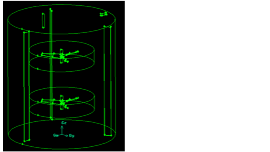
Figure 1. Schematic diagram of computational domain.
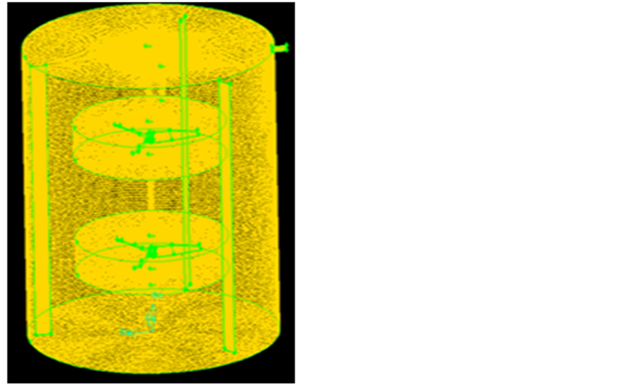
Figure 2. Meshed geometry.
tinues the upward movement and then returns downwards to rejoin the flow.
It is observed that fluid circulation results in vortex (circulation loops) formation where two types of circulation loops can be identified in the flow field. They consist of a strong primary loop in the impeller discharge region and a smaller secondary loop below the impeller. Usually, the flow field generated by down-pumping multiple impellers with large values of impeller separation (also known as S/H values) is such that the downward discharge and circulation loops are well defined for each impeller as in studies conducted by [25] [26] . However,
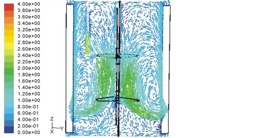
Figure 3. Flowfield in the (r-z) vertical plane at 0˚.
in the present study, it is observed that the loops are more pronounced in the discharge region of the lower impeller. This can be explained by the short separation between the two impellers which resulted in a strong interaction of their active volumes. In this case, the downward discharge flow of the upper impeller is picked up by the lower impeller.
The circulation loops clearly show flow segregation within the tank and therefore confirms the tanks-in-series with exchange model which was found suitable to describe the flow structure in the leaching tanks in the experimental investigation of Dagadu et al. (2011).
3.2. Flow Distribution
A representative velocity contour plot describing the flow distribution in the tank is shown in Figure 4. It is observed that the distribution of liquid velocity differs significantly in the flow domain where the highest velocity magnitude is observed at the impeller tips. Thus, indicating uneven distribution of ore slurry in the tank. Low material concentration is observed mainly at the top and around the central axis near the bottom of tank. The central portion of the vortex regions also indicates low material concentration which confirms the fact that the speed of a forced (rotational) vortex is zero at the centre and increases proportionally to the distance from the centre.
The main concern of solid-liquid stirred tanks is the build-up solids on the tank bottom over time. In this study the contour plots revealed that the tank exhibit good Off-Bottom Suspension. The strong tangential velocity component keeps the solids suspended off the tank bottom and will not accumulate over time. This is very important for gold leaching tanks where the efficiency of gold recovery could be reduced significantly due to build-up of gold ore particles on the bottom of the leaching tanks.
This study has shown that due to the low speed of agitation employed in gold leaching tanks it better to design down-pumping multiple impellers with relatively small values of impeller separation in order to prevent solid build-up on the bottom of tanks. If the separation is large the discharge from the upper impeller may not be picked-up the lower impeller to send a strong downward discharge and keep the solids suspended off the tank bottom.
4. Conclusions
CFD codes were used to simulate the flow pattern of a representative leaching tank using an Eulerian-Eulerian multi-fluid model. Additionally, the RANS standard k-ε mixture model and a multiple reference frame approach were used to model turbulence and impeller rotation respectively. The main conclusions drawn from the inves-
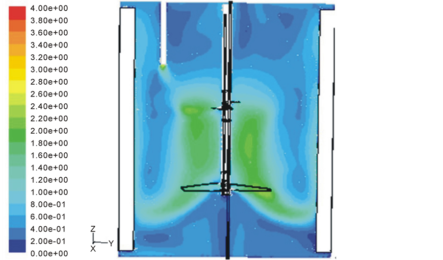
Figure 4. Contours of velocity magnitude.
tigation are as follows:
Ÿ Flow distribution, in the simulated flowfield, was found to be in agreement with the flow pattern generated by the pitched blade axial-flow impellers that was used for mixing.
Ÿ Circulation loops within the flowfield resulted in flow segregation within the tank and confirms the tanks-inseries with exchange model which was used to describe the flow structure in the leaching tanks in a tracer experiment conducted earlier.
Ÿ Velocity contour plots reveal minimum deposition of gold ore particles on the bottom of the leaching tanks due to the strong tangential velocity component, of the lower impeller discharge.
Ÿ In general, the CFD approach gave a better description of the flow structure in a leaching tank and could therefore be used for industrial flow analysis instead of experimental methods that are not only cost intensive but also do not provide any clear picture of the flowfield. The CFD approach is necessary for effective design of flow systems and validation of design data especially after process intensification.
Acknowledgements
The authors are indebted to Abosso Goldfields Ghana Limited, Damang Processing Plant, for providing technical information on plant design. We are also grateful to the International Atomic Energy Agency for financial support. This work was also supported by the Polish Committee for Scientific Research.
References
- Delvigne, F., Destain, J. and Thonart, P. (2005) Structured Mixing Model for Stirred Bioreactors: An Extension to the Stochastic Approach. Chemical Engineering Journal, 113, 1-12. http://dx.doi.org/10.1016/j.cej.2005.06.007
- Raju, R., Balachandar, S., Hill, D.F. and Adriana, R.J. (2005) Reynolds Number Scaling of Flow in a Stirred Tank with Rushton Turbine. Part II—Eigen Decomposition of Fluctuation. Chemical Engineering Science, 60, 3185-3198. http://dx.doi.org/10.1016/j.ces.2004.12.040
- Yoon, H.S., Sharp, K.V., Hill, D.F., Adrian, R.J., Balachandar, S., Ha, M.Y. and Kar, K. (2001) Integrated Experimental and Computational Approach to Simulation of Flow in a Stirred Tank. Chemical Engineering Science, 56, 6635-6649. http://dx.doi.org/10.1016/S0009-2509(01)00315-3
- Vakili, M.H. and Esfahany, M.N. (2009) CFD Analysis of Turbulence in a Baffled Stirred Tank, a Three-Compartment Model. Chemical Engineering Science, 64, 351-362. http://dx.doi.org/10.1016/j.ces.2008.10.037
- Wang, Z., Mao, Z. and Shen, X. (2006) Numerical Simulation of Macroscopic Mixing in a Rushton Impeller Stirred Tank. The Chinese Journal of Process Engineering, 6, 857-863.
- Lelinski, D., Allen, J., Redden, L. and Weber, A. (2002) Analysis of the Residence Time Distribution in Large Flotation Machines. Minerals Engineering, 15, 499-505. http://dx.doi.org/10.1016/S0892-6875(02)00070-5
- Furman, L. and Stegowski, Z. (2011) CFD Models of Jet Mixing and Their Validation by Tracer Experiments. Chemical Engineering and Processing, 50, 300-304. http://dx.doi.org/10.1016/j.cep.2011.01.007
- Murthy, B.N., Ghadge, R.S. and Joshi, J.B. (2007) CFD Simulations of Gas-Liquid-Solid Stirred Reactor: Prediction of Critical Impeller Speed for Solid Suspension. Chemical Engineering Science, 62, 7184-7195. http://dx.doi.org/10.1016/j.ces.2007.07.005
- Panneerselvam, R., Savithri, S. and Surender, G.D. (2008) CFD Modeling of Gas-Liquid-Solid Mechanically Agitated Contactor. Chemical Engineering Research and Design, 8, 1331-1344. http://dx.doi.org/10.1016/j.cherd.2008.08.008
- Deglon, D.A. and Meyer, C.J. (2006) CFD Modelling of Stirred Tanks: Numerical Considerations. Minerals Engineering, 19, 1059-1068. http://dx.doi.org/10.1016/j.mineng.2006.04.001
- Meroney, R.N. and Colorado, P.E. (2009) CFD Simulation of Mechanical Draft Tube Mixing in Anaerobic Digester Tanks. Water Research, 43, 1040-1050. http://dx.doi.org/10.1016/j.watres.2008.11.035
- Angst, R., Harnack, E., Singh, M. and Kraume, M. (2003) Grid and Model Dependency of the Solid/Liquid Two-Phase Flow CFD Simulation of Stirred Reactors. Proceedings of 11th European Conference of Mixing, Bambarg, 14-17 October 2003.
- Barrue, H., Bertrand, J., Cristol, B. and Xuereb, C. (2001) Eulerian Simulation of Dense Solid-Liquid Suspension in Multi-Stage Stirred Reactor. Journal of Chemical Engineering of Japan, 34, 585-594. http://dx.doi.org/10.1252/jcej.34.585
- Lopez de Bertodano, M. (1992) Turbulent Bubbly Two-Phase Flow in a Triangular Duct. Ph.D. Dissertation, Rensselaer Polytechnic Institute, Troy, New York.
- Cheung, S.C.P., Yeoh, G.H. and Tu, J.Y. (2007) On the Modelling of Population Balance in Isothermal Vertical Bubbly Flows-Average Bubble Number Density Approach. Chemical Engineering Process, 46, 742-756. http://dx.doi.org/10.1016/j.cep.2006.10.004
- Lucas, D., Kreppera, E. and Prasserb, H.M. (2007) Use of Models for Lift, Wall and Turbulent Dispersion Forces Acting on Bubbles for Poly-Disperse Flows. Chemical Engineering Science, 62, 4146-4157. http://dx.doi.org/10.1016/j.ces.2007.04.035
- Khopkar, A.R., Rammohan, A.R., Ranade, V.V. and Dudukovic, M.P. (2005) Gas-Liquid Flow Generated by a Rushton Turbine in Stirred Vessel: CARPT/CT Measurement and CFD Simulations. Chemical Engineering Science, 60, 2215-2229. http://dx.doi.org/10.1016/j.ces.2004.11.044
- Montante, G. and Magelli, F. (2005) Modelling of Solids Distribution in Stirred Tanks: Analysis of Simulation Strategies and Comparison with Experimental Data. International Journal of Computational Fluid Dynamics, 19, 253-262. http://dx.doi.org/10.1080/10618560500081795
- Brucato, A., Grisafi, F. and Montante, G. (1998) Particle Drag Coefficient in Turbulent Fluids. Chemical Engineering Science, 45, 3295-3314. http://dx.doi.org/10.1016/S0009-2509(98)00114-6
- Khopkar, A.R. and Tanguy, P.A. (2008) CFD Simulation of Gas-Liquid Flows in Stirred Vessel Equipped with Dual Rushtonturbines: Influence of Parallel, Merging and Diverging Flow Configurations. Chemical Engineering Science, 63, 3810-3820. http://dx.doi.org/10.1016/j.ces.2008.04.039
- Aubin, J., Kresta, S.M., Bertrand, J., Xuereb, C. and Fletcher, D.F. (2006) Alternate Operating Methods for Improving the Performance of Continuous Stirred Tank Reactors. Chemical Engineering Research and Design, 84, 569-582. http://dx.doi.org/10.1205/cherd.05216
- Khopkar, A.R., Mavros, P., Ranade, V.V. and Bertrand, J. (2004) Simulation of Flow Generated by an Axial Flow Impeller: Batch and Continuous Operation. Chemical Engineering Research and Design, 82, 737-751. http://dx.doi.org/10.1205/026387604774196028
- ANSYS FLUENT Inc. (2006) FLUENT 6.3 User’s Manual. Fluent Inc. Centrera Resource Park, 10 Cavendish Court, Lebanon.
- Vasquez, S.A. and Ivanov, V.A. (2000) A Phase Coupled Method for Solving Multiphase Problems on Unstructured Meshes. Proceedings of the ASME Fluids Engineering Division Summer Meeting (FEDSM2000), American Society of Mechanical Engineers, 251, 659-664.
- Bai, H., Stephenson, A., Jimenez, J., Jewell, D. and Gillis, P. (2008) Modeling of Flow and Residence Time Distribution in an Industrial-Scale Reactor with a Plunging Jet Inlet and Optional Agitation. Chemical Engineering Research and Design, 8, 1462-1476. http://dx.doi.org/10.1016/j.cherd.2008.08.012
- Jahoda, M., Mostek, M., Kukukova, K.A. and Machon, V. (2007) CFD Modelling of Liquid Homogenization in Stirred Tanks with One and Two Impellers Using Large Eddy Simulation. Chemical Engineering Research and Design, 85, 616-625. http://dx.doi.org/10.1205/cherd06183
NOTES

*Corresponding author.