International Journal of Intelligence Science
Vol.3 No.1A(2013), Article ID:29548,13 pages DOI:10.4236/ijis.2013.31A007
Rough Mereology as a Tool for Knowledge Discovery and Reasoning in Intelligent Systems: A Survey
Computer Science Department, Polish-Japanese Institute of Information Technology, Warszawa, Poland
Email: polkow@pjwstk.edu.pl
Received October 24, 2012; revised November 28, 2012; accepted December 12, 2012
Keywords: Knowledge Engineering; Rough Mereology; Granular Computing; Data Mining; Intelligent Robotics
ABSTRACT
In this work, we present an account of our recent results on applications of rough mereology to problems of 1) knowledge granulation; 2) granular preprocessing in knowledge discovery by means of decision rules; 3) spatial reasoning in multi-agent systems in exemplary case of intelligent mobile robotics.
1. Introduction the Tool: Rough Mereology
Rough Mereology (RM, for short) is a paradigm in the domain of Approximate Reasoning, which is an extension of Mereology, see [1-3]. RM is occupied with a class of similarity relations among objects which are expressed as rough inclusions, see [4-8]. A rough inclusion is a ternary predicate , read as: The object x is a part in object y to a degree of
 . For a detailed discussion of rough inclusions along with an extensive historic bibliography, see [8].
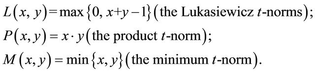
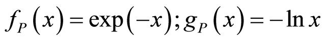
Rough inclusions can be induced from continuous tnorms, see [8,9] whose classical examples are
Rough inclusions can be obtained from residual implications  cf. [9], induced by continuous t-norms as 1.1.1.
 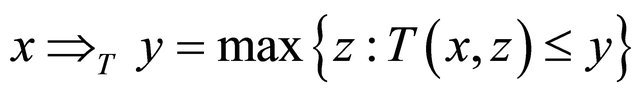 (1)
(1)
Then,
 (2)
(2)
is a rough inclusion. A particular case of continuous tnorms are Archimedean t-norms which satisfy the inequality  for each
 . It is wellknown, cf. [8,9], that each Archimedean t-norm T admits a representation
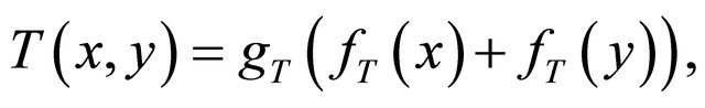 (3)
(3)
where the function 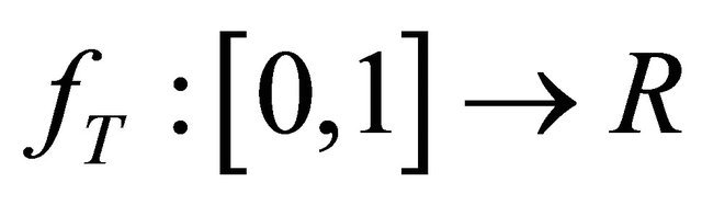 is continuous decreasing with
 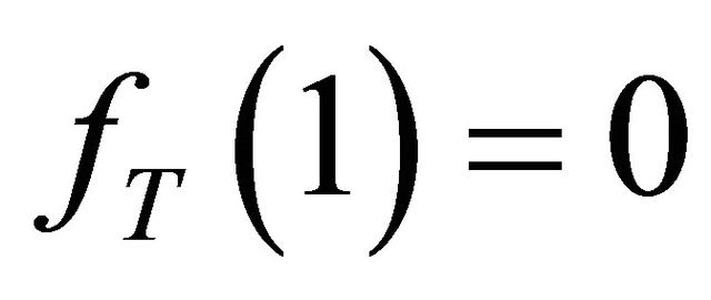 and
and  is the pseudo-inverse to fT, i.e.,
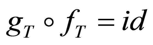 . There are two basic Archimedean t-norms: L and P. Their representations are 1.1.2.
 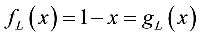 (4)
(4)
and
 (5)
(5)
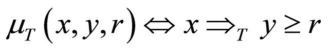
For an Archimedean t-norm T, we define the rough inclusion µT on the interval [0,1] by means of 1.1.3. 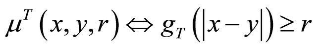 (6)
(6)
Specific recipes are 1.1.4. 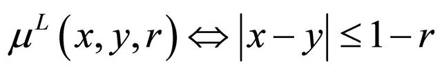 (7)
(7)
and
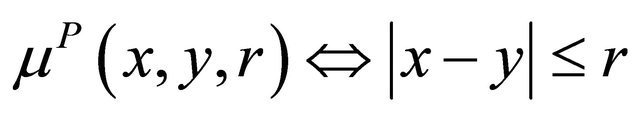 (8)
(8)
Both residual and Archimedean rough inclusions satisfy the transitivity condition, see [8]
(Trans) if  then
then 
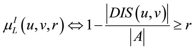
An important domain where rough inclusions play a dominant role in our mining of knowledge is the realm of information/decision systems in the sense of Pawlak, cf., [8,10]. For a recent view on information systems in a broader perspective of applications, see [11]. We will define information rough inclusions denoted with a generic symbol . We recall that an information system (a data table) is represented as a pair
  where U is a finite set of objects and A is a finite set of attributes; each attribute a:
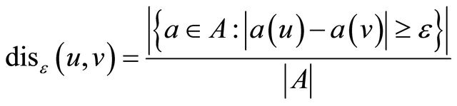
  maps the set U into the value set V. A decision system adds to the set A of attributes an attribute called decision d not in A. For objects u, v the discernibility set
  is defined as
 (9)
(9)
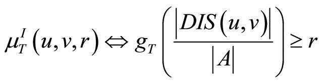
For a rough inclusion of the form µT, we define a rough inclusion  by means of
 (10)
(10)
Then,  is a rough inclusion with the associated ingredient relation of identity and the part relation empty. For the Łukasiewicz t-norm, the rough inclusion
  is given by means of the formula, cf. [8]
 (11)
(11)
We introduce the set 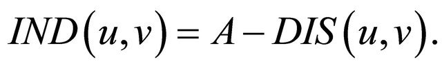 With its help a new form of (11) is 1.1.5.
 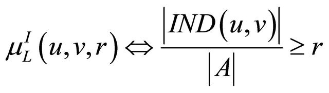 (12)
(12)
Formula (12) witnesses that reasoning based on the rough inclusion  is the probabilistic one. Rough inclusions of type
  satisfy the transitivity condition (Trans) and are symmetric. Formula (12) can be abstracted for set and geometric domains. For finite sets A, B, we let 1.1.6.
 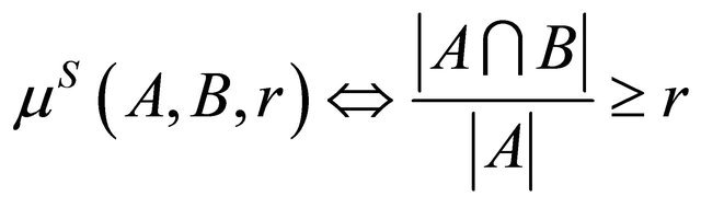 (13)
(13)
where  denotes the cardinality of the set X. For bounded measurable sets A, B in an Euclidean space
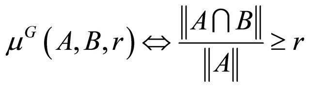 (14)
(14)
defines a rough inclusion µG, where  is the area (Lebesgue measure) of X. Both µS and µG are symmetric but not transitive. Default value is 1 in case A is empty or of measure 0.
2. Granulation of Knowledge
Granular computing goes back to Lotfi A. Zadeh and its idea lies in aggregating objects with respect to a chosen similarity measure into “granules” of satisfactorily similar objects, see [5,6,8,12,13].
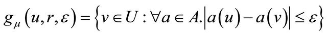
For a given rough inclusion μ, the granule  of the radius r about the center u is defined as the class of property
 (15)
(15)
where
 (16)
(16)
Hence, an object v belongs in the granule  if and only if
 .
.
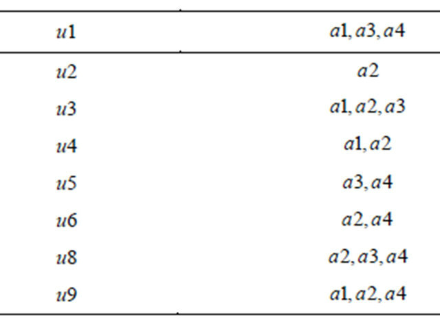
For the exemplary information system in Table 1 with attributes , and objects u1 to u9, we can compute granules with respect to, for instance,
 . Table 2 shows the values of sets
  for
for ; the set
  is omitted as it includes all attributes.
Clearly, granules of all radii between 0 and 1 about all objects in a given universe U, provide a quasi-metric topology on U.
3. Mereogeometry
Quasi-metric topology mentioned above may be applied in the build-up of mereogeometry, cf. [8,14,15]. Elementary geometry was defined by Tarski as a part of Euclidean geometry which can be described by means of 1st order logic. There are two main aspects in formalization of geometry: one is metric aspect dealing with the distance underlying the space of points which carries geometry and the other is affine aspect taking into account linear relations. In the Tarski axiomatization for 2- and 3-dimensional elementary geometry, recalled in [8], the metric aspect is expressed as a relation of equidistance (a congruence) and the affine aspect is expressed by means
Table 1. An information system A.
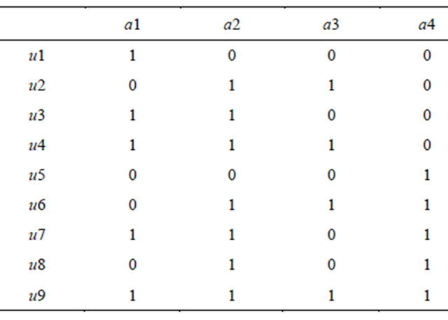
Table 2. Sets  for the system A.
of the betweenness relation. The only logical predicate required is the identity “=”. Equidistance relation denoted 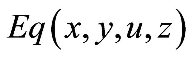 (or, as a congruence:
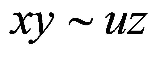 ) means that the distance from x to y is equal to the distance from u to z (pairs x, y and u, z are equidistant). Betweenness relation is denoted
 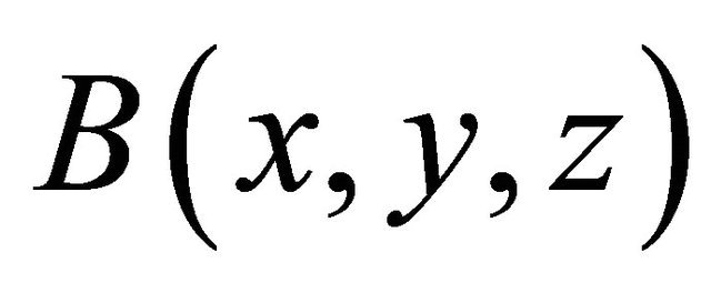 (x is between y and z). Van Benthem [16] took up the subject proposing a version of betweenness predicate based on the nearness predicate and suited, hypothetically, for Euclidean spaces. We are interested in introducing into the mereological world defined by
  of a geometry in whose terms it will be possible to express spatial relations among objects. We first introduce a notion of a distance
 , induced by a rough inclusion
 ,
,
 (17)
(17)
Observe that the mereological distance differs essentially from the standard distance: the closer are objects, the greater is the value of  means X = Y whereas
  means that X,Y are either externally connected or disjoint, no matter what is the Euclidean distance between them. We use
  to define in our context the relation N of nearness proposed in [16]:
 (18)
(18)
Here,  means that X is closer to U than V is to U. We introduce a betweenness relation in the sense of Van Benthem TB modeled on betweenness proposed in [16]:
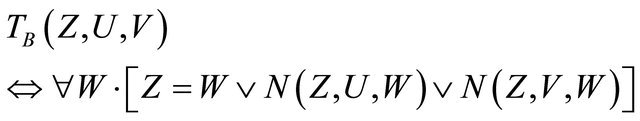 (19)
(19)
The principal example bearing, e.g., on our approach to robot control deals with rectangles in 2D space regularly positioned, i.e., having edges parallel to coordinate axes. We model robots (which are represented in the plane as discs of the same radii in 2D space) by means of their safety regions about robots; those regions are modeled as squares circumscribed on robots. One of advantages of this representation is that safety regions can be always implemented as regularly positioned rectangles. Given two robots a, b as discs of the same radii, and their safety regions as circumscribed regularly positioned rectangles A, B, we search for a proper choice of a region X containing A and B with the property that a robot C contained in X can be said to be between A and B. In this search we avail ourselves with the notion of betweenness relation TB.
Taking the rough inclusion  defined in (14), for two disjoint rectangles A,B, we define the extent,
  , of A and B, as the smallest rectangle (the convex hull) containing the union
 . Then we have the claim: the only object between C and D in the sense of the predicate TB is the extent
 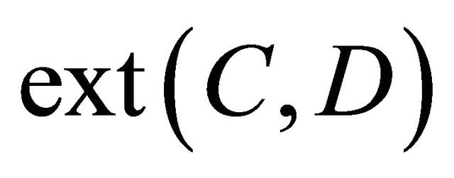 of C and D.
For a proof, as linear stretching or contracting along an axis does not change the area relations, it is sufficient to consider two unit squares A, B of which A has  as one of vertices whereas B has
  with
with  as the lower left vertex (both squares are regularly positioned).
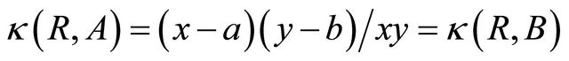
Then the distance κ between the extent  and either of A, B is
 . For a rectangle
 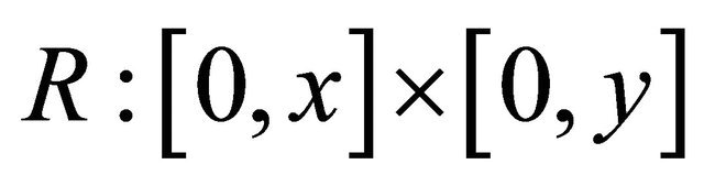 with x in
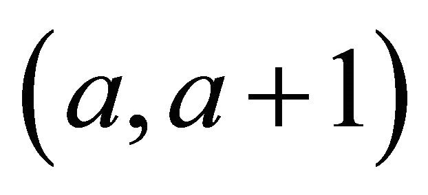 , y in
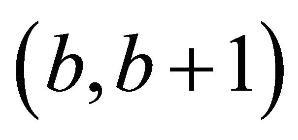 , we have that
 (20)
(20)
For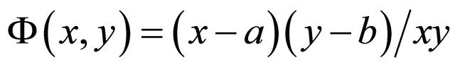 , we find that
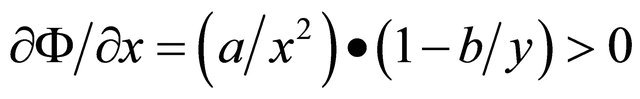 (21)
(21)
and, similarly,  , i.e., Ф is increasing in x, y reaching the maximum when R becomes the extent of A, B.
We return to this result when we discuss planning and navigation problems in behavioral robotics for teams of autonomous mobile robots.
4. Rough Mereology in Behavioral Robotics
Planning is concerned with setting a trajectory for a robot endowed with some sensing devices which allow it to perceive the environment in order to reach by the robot a goal in the environment at the same time bypassing obstacles.
A method of potential field, see [17] consists in constructing a potential field composed of attractive potentials for goals and repulsive potentials for obstacles. In [14,15,18] a mereological potential field planning method was proposed. Classical methodology of potential fields works with integrable force field given by formulas of Coulomb or Newton which prescribe force at a given point as inversely proportional to the squared distance from the target; in consequence, the potential is inversely proportional to the distance from the target.
The basic property of the potential is that its density (=force) increases in the direction toward the target. We observe this property in our construction. We apply the geometric rough inclusion
 (22)
(22)
where  is the area of the region x. In our construction of the potential field, region will be squares: robots are represented by squares circumscribed on them (simulations were performed with disk-shaped Roomba robots, the intellectual property of iRobot Inc.).
Geometry induced by means of a rough inclusion can be used to define a generalized potential field: the force field in this construction can be interpreted as the density of squares that fill the workspace and the potential is the integral of the density. We present now the details of this construction.
We construct the potential field by a discrete construction. The idea is to fill the free workspace of a robot with squares of fixed size in such a way that the density of the square field (measured, e.g., as the number of squares intersecting the disc of a given radius r centered at the target) increases toward the target. To ensure this property, we fix a real number, the field growth step in the interval (0, square edge length); in our exemplary case the parameter field growth step is set to 0.01. The collection of squares grows recursively with the distance from the target by adding to a given square in the  -th step all squares obtained from it by translating it by k• field growth step (with respect to Euclidean distance) in basic eight directions: N, S, W, E, NE, NW, SE, SW (in the implementation of this idea, the floodfill algorithm with a queue has been used, see [18]. Once the square field is constructed, the path for a robot from a given starting point toward the target is searched for. The idea of this search consists in finding a sequence of waypoints which delineate the path to the target. Way-points are found recursively as centroids of unions of squares mereologically closest to the square of the recently found way-point. In order to define the potential of the rough mereological field, let us consider how many generations of squares will be centered within the distance r from the target. Clearly, we have
 (23)
(23)
where d is the field growth step, k is the number of generations. Hence,
 (24)
(24)
and thus
 (25)
(25)
The potential  can be taken as
 . The force field
  is the negative gradient of
 ,
,
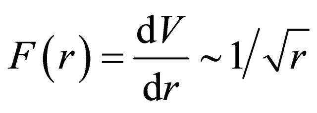 (26)
(26)
Hence, the force decreases with the distance r from the target slower than traditional Coulomb force. It has advantages of slowing the robot down when it is closing on the target. Parameters of this procedure are: the field growth step set to 0.01, and the size of squares which in our case is 1.5 times the diameter of the Roomba robot.
A view of mereological potential field is given in Figure 1.
A robot should follow the path proposed by planner shown in Figure 2.
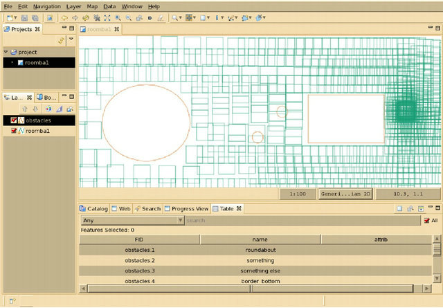
Figure 1. Mereological potential field.

Figure 2. Paths planned for robots to the goal.
Rough Mereological Approach to Robot Formations
We recall that on the basis of the rough inclusion μ, and mereological distance κ, geometric predicates of nearness and betweenness, are redefined in mereological terms. Given two robots a, b as discs of same radii, and their safety regions as circumscribed regularly positioned rectangles A, B, we search for a proper choice of a region X containing A and B with the property that a robot C contained in X can be said to be between A and B. We recall that the only object X with these property is the extent , i.e., the minimal rectangle containing the union
 , i.e., the convex hull of the union
 . For details of the exposition which we give now, please consult [19,20]. For robots a, b, c, we say that the robot b is between robots a and c, in symbols
 (27)
(27)
in case the rectangle  is contained in the extent of
 , i.e.1.1.7.
  (28)
(28)
This allows as well for a generalization of the notion of betweenness to the notion of partial betweenness which models in a more realistic manner spatial relations among a, b, c; we say in this case that the robot b is between robots a and c to a degree of at least r, in symbols,
 , (29)
i.e.1.1.8.  (30)
(30)
For a team of robots,  , an ideal formation IF on T is a betweenness relation (between...) on the set T of robots. In implementations, ideal formations are represented as lists of expressions of the form
 (31)
(31)
indicating that the object r0 is between r1, r2, along with a list of expressions of the form
 (32)
(32)
indicating triples which are not in the given betweenness relation. To account for dynamic nature of the real world, in which due to sensory perception inadequacies, dynamic nature of the environment, etc., we allow for some deviations from ideal formations by allowing that the robot which is between two neighbors can be between them to a degree in the sense of (29). This leads to the notion of a real formation. For a team of robots,  , a real formation RF on T is a betweenness to degree relation (betweendeg...) on the set T of robots. In practice, real formations will be given as a list of expressions of the form,
 (33)
(33)
indicating that the object r0 is to degree of δ in the extent of r1, r2, for all triples in the relation (between—deg...), along with a list of expressions of the form,
 (34)
(34)
indicating triples which are not in the given betweenness relation.
Description of formations, as proposed above, can be a list of relation instances of large cardinality, cf., examples below. The problem can be posed of finding a minimal set of instances sufficient for describing a given formation, i.e., implying the full list of instances of the relation . This problem turns out to be NPhard, see [20]. To describe formations we have proposed a language derived from LISP-like s-expressions: a formation is a list in LISP meaning with some restricttions that delimit our language. We will call elements of the list objects. Typically, LISP lists are hierarchical structures that can be traversed using recursive algorithms. We assume that top-level list (a root of whole structure) contains only two elements where the first element is always a formation identifier (a name). For instance(formation1(some—predicate param1... paramN))
For each object on a list (and for a formation as a whole) an extent can be derived and in facts, in most cases only extents of those objects are considered. We have defined two possible types of objects: 1) Identifier: robot or formation name (where formation name can only occur at top-level list as the first element); 2) Predicate: a list in LISP meaning where first element is the name of given predicate and other elements are parameters; number and types of parameters depend on given predicate. Minimal formation should contain at least one robot. For example(formation2 roomba0)
To help understand how predicates are evaluated, we need to explain how extents are used for computing relations between objects. Suppose we have three robots (roomba0, roomba1, roomba2) with roomba0 between roomba1 and roomba2 (so the  predicate is satisfied). We can draw an extent of this situation as the smallest rectangle containing the union
  oriented as a regular rectangle, i.e., with edges parallel to coordinate axes. This extent can be embedded into bigger structure: it can be treated as an object that can be given as a parameter to predicate of higher level in the list hierarchy. For example, cf. Figure 3(formation3 (between (between roomba0 roomba1 roomba2) roomba3 roomba4))
We can easily find more than one situation of robots that fulfill this example description. That is one of the features of our approach: one s-expression can describe many situations. This however makes very hard to find minimal s-expression that would describe already given arrangement of robots formation (as stated earlier in this chapter, the problem is NP-hard). Typical formation description may look like below, see [19],
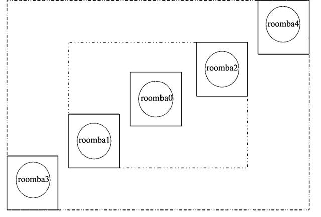
Figure 3. Extents of roombaTM robots.
(cross
(set
(max—dist 0.25 roomba0 (between roomba0 roomba1 roomba2))
(max—dist 0.25 roomba0 (between roomba0 roomba3 roomba4))
(not—between roomba1 roomba3 roomba4)
(not—between roomba2 roomba3 roomba4)
(not—between roomba3 roomba1 roomba2)
(not—between roomba4 roomba1 roomba2)
)
)
This is a description of a formation of five Roomba robots arranged in a cross shape. The max-dist relation is used to bound formation in space by keeping all robots close one to another. We show a screen-shot of robots (submittted by Dr Paul Osmialowski) in the initial formation of cross-shape in a crowded environment, see Figures 4 and 5. These behaviors witness the flexibility of our definition of a robot formation: first, robots can change formation, next, as the definition of a formation is
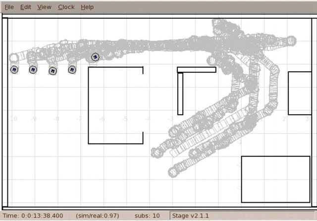
Figure 4. Trails of robots in the line formation through the passage.
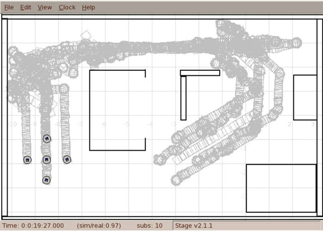
Figure 5. Trails of robots in the restored cross formation after passing through the passage.
relational, without metric constraints on robots, the formation can manage an obstacle without losing the prescribed formation (though, this feature is not illustrated in figures in this chapter).
5. Granular Classifiers
We recall that for a decision system  with the decision d, a decision rule is an implication 1.1.9.
  (35)
(35)
where  is a set of attributes, va is a value of the attribute a; the formula
  is the descriptor whose meaning is the set
 ; these elementary meanings define the meaning of the formula r by interpreting the disjunction
  of descriptors as the union
  of meanings, the conjunction
  of descriptors as the intersection
  of meanings. Coefficients of accuracy and coverage are defined for a decision algorithm D, trained on a training set Tr and tested on a test set Tst, as, respectively, quotients 1.1.10.
1.1.11. where ncorr is the number of test objects correctly classified by D and ncaught is the number of test objects classified, and,

where ntest is the number of test objects. Thus, the product
gives the measure of the fraction of test objects correctly classified by D. We have already mentioned that accuracy and coverage are often advised to be combined in order to better express the trade-off between the two: one may have a high accuracy on a relatively small set of caught objects, or a lesser accuracy on a larger set of caught by the classifier objects. Michalski [21] proposes a combination rule of the form 1.1.12. 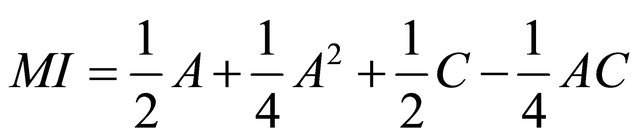 (36)
(36)
where A stands for accuracy and C for coverage. With the symbol MI, we denote the Michalski index as defined in (36).
5.1. The Idea of Granular Rough Mereo-Logical Classifiers
Our idea of augmenting existing strategies for rule induction consists in using granules of knowledge. The principal assumption we can make is that the nature acts in a continuous way: if objects are similar with respect to judiciously and correctly chosen attributes, then decisions on them should also be similar. A granule collecting similar objects should then expose the most typical decision value for objects in it while suppressing outlying values of decision, reducing noise in data, hence, leading to a better classifier. The idea of a rough mereological granular classifier was proposed and refined in [22,23]. We give a resume of the most important ideas and results in this area. We assume that we are given a decision system  from which a classifier is to be constructed; for a discussion on the subject of data classification, cf., e.g. [24]; we assume that on the universe U, a rough inclusion μ is given, and a radius r in [0,1] is chosen, consult [8] for detailed discussion. We can find granules
  for all u in U, and make them into the set
 . From this set, a covering
  of the universe U can be selected by means of a chosen strategy
 , i.e.,
 (37)
(37)
We intend that  becomes a new universe of the decision system whose name will be the granular reflection of the original decision system. It remains to define new attributes for this decision system. Each granule g in
  is a collection of objects; attributes in the set
  can be factored through the granule g by means of a chosen strategy
 , i.e., for each attribute q in
 , the new factored attribute 1.1.13.
  (38)
(38)
is defined. In effect, a new decision system
 (39)
(39)
is defined. The object vg with values  is called the granular reflection of the granule g. Granular reflections of granules need not be objects found in data set; yet, the results show that they mediate very well between the training and test sets. We include in Table 3 the granular reflection of the system
 , shown in Table 1, for the radius r = 0.75. We select the covering
  sequentially: assuming that elements
  of this covering are selected already, the element
  is selected as the granule of the least cardinality such that it does intersect the set
  on the set of the largest cardinality, with random tie resolution. A look at Table 4 convinces us that the set
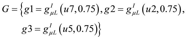
can be taken as the covering. As the strategy  we adopt the majority voting. On the basis, again, of Table 4, and of the strategy
 , we find the granular reflection
 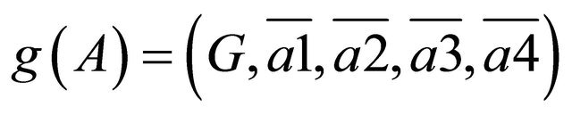 shown in Table 3.
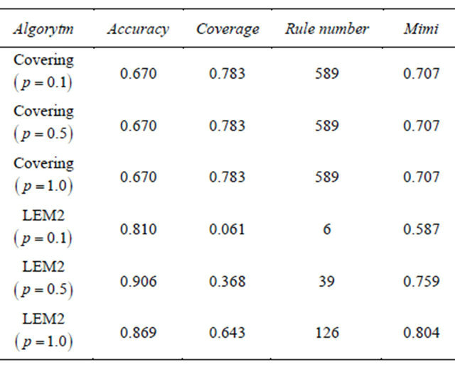
In order to demonstrate results of this approach on real data, we consider a standard data set the Australian Credit Data Set from University of California at Irvine Machine Learning Repository and we collect the best results for this data set by various rough set based methods in Table 5; they come from works by Bazan [25], Sinh Hoa Nguyen [26], and Wroblewski [27]. For a comparison we include in Table 6 results obtained by some other methods, as given in Statlog. In Table 7, we give a comparison of performance of rough set classifiers: exhaustive, covering and LEM, cf. [24], implemented in the Rough Set Exploratory System (RSES) due to Skowron et al. [28]. We begin in the next section with granular classifiers in which granules are induced from the training set, cf. [29-32].
Table 3. Granular reflection g(A).
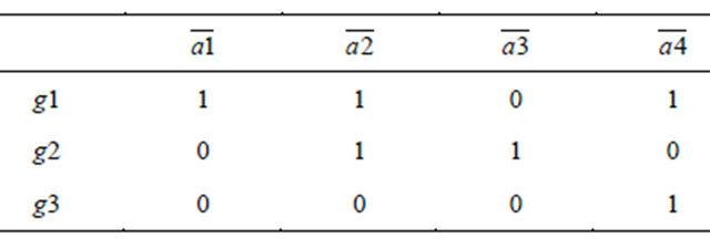
Table 4. Granules  for the system A.
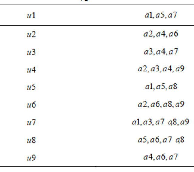
Table 5. Best results for Australian credit by some rough set based algorithms.
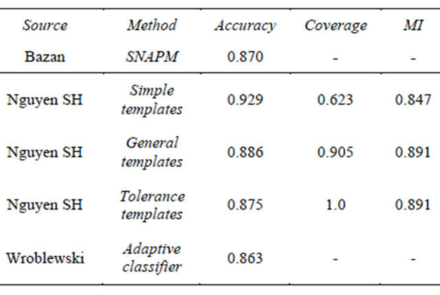
Table 6. A comparison of errors in classification by rough set and other paradigms.
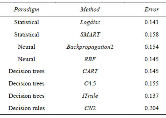
Table 7. Train and test (trn = 345 objects, tst = 345 objects); Australian credit; comparison of RSES implemented algorithms: exhaustive, covering and LEM.
5.2. Classification by Granules of Training Objects
We begin with a classifier in which granules computed by means of the rough inclusion μL form a granular reflection of the data set and then to this new data set the exhaustive classifier available in RSES is applied.
Procedure of the Test
1) The data set  is input;
2) The training set is chosen at random. On the training set, decision rules are induced by means of exhaustive, covering and LEM algorithms implemented in the RSES system;
3) Classification is performed on the test set by means of classifiers of pt. 2;
4) For consecutive granulation radii r, granule sets  are found;
5) Coverings  are found by a random irreducible choice;
6) For granules in , for each r, we determine the granular reflection by factoring attributes on granules by means of majority voting with random resolution of ties;
7) For found granular reflections, classifiers are induced by means of algorithms in pt. 2;
8) Classifiers found in pt. 7, are applied to the test set;
9) Quality measures: accuracy and coverage for classifiers are applied in order to compare results obtained, respectively, in pts. 3 and 8.
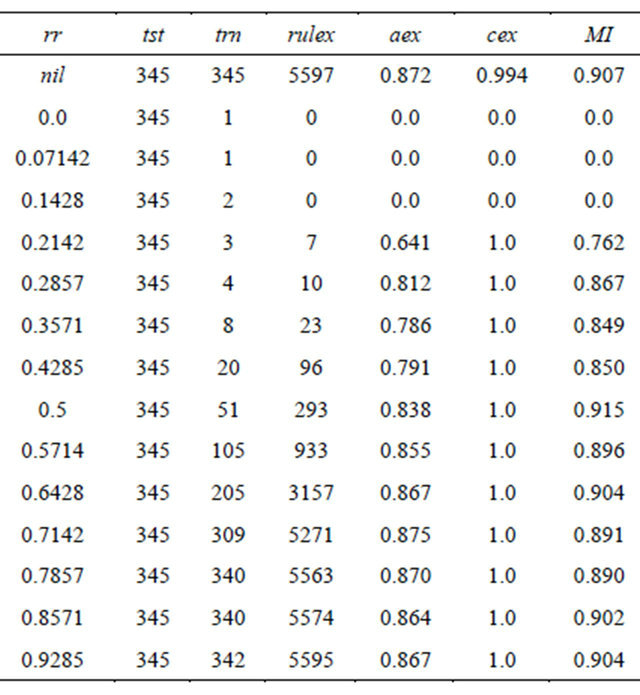
In Table 8, the results are collected obtained after the procedure described above is applied.
We can compare results expressed in terms of the Michalski index MI as a measure of the trade-off between accuracy and coverage; for template based methods, the best MI is 0.891, for covering or LEM algorithms the best value of MI is 0.804, for exhaustive classifier  MI is equal to 0.907 and for granular reflections, the best MI value is 0.915 with few other values exceeding 0.900. What seems worthy of a moment’s reflection is the number of rules in the classifier. Whereas for the exhaustive classifier
  in nongranular case, the number of rules is equal to 5597, in granular case the number of rules can be surprisingly small with a good MI value, e.g., at r = 0.5, the number of rules is 293, i.e., 5 percent of the exhaustive classifier size, with the best MI of all of 0.915. This compression of classifier seems to be the most impressive feature of granular classifiers. This initial, simple granulation, suggests further ramifications. For instance, one can consider, for a chosen value of ε in [0,1], granules of the form.
Table 8. Train and test; Australian credit; granulation for rdii r; RSES exhaustive classifier; r = granule radius; tst = test set size; trn = training set size; rulex = rule number; aex = accuracy; cex = coverage.
and repeat with these granules the procedure of creating a granular reflection and building from it a classifier. Another yet variation consists in mimicking the performance of the Łukasiewicz based rough inclusion and introducing a counterpart of the granulation radius in the form of the catch radius, . The granule is then dependent on two parameters: ε and
  and its form is 1.1.14.
 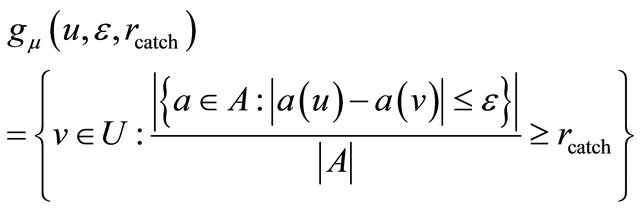 (40)
(40)
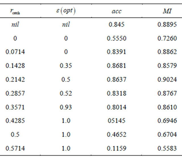
Results of classification by granular classifier induced from the granular reflection obtained by means of granules (39) are shown in Table 9.
5.3. A Treatment of Missing Values
A particular but important problem in data analysis is the treatment of missing values. In many data, some values of some attributes are not recorded due to many factors, like omissions, inability to take them, loss due to some events etc. Our idea is to embed the missing value into a granule: by averaging the attribute value over the granule in the way already explained, it is hoped the the average value would fit in a satisfactory way into the position of the missing value. We will use the symbol *, commonly used for denoting the missing value; we will use two methods for treating *, i.e, (1) either * is a don’t care symbol meaning that any value of the respective attribute can be substituted for *, hence, * = v for each value v of the attribute, or (2) * is a new value on its own, i.e., if * = v
Table 9. Classification with granules of the form (39). ε(opt) = optimal value of ε; acc = accuracy; cov = coverage. Best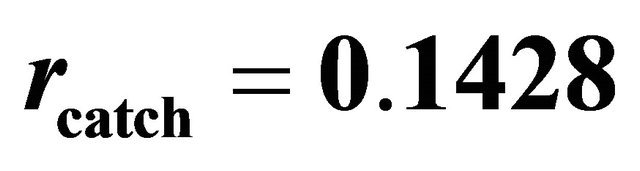 ,
,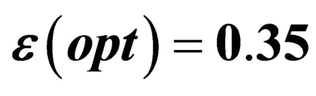 ; best accuracy = 0.8681, coverage = 1.
then v can only be *; see [33] for a general discussion on the missing data problem. Our procedure for treating missing values is based on the granular structure ; the strategy
  is the majority voting, i.e., for each attribute a, the value
  is the most frequent of values in
 . The strategy
  consists in random selection of granules for a covering. For an object u with the value of * at an attribute a, and a granule
  in
in , the question whether u is included in g is resolved according to the adopted strategy of treating *: in case * = don’t care, the value of * is regarded as identical with any value of a, hence,
  is automatically increased by 1, which increases the granule; in case * = *, the granule size is decreased. Assuming that * is sparse in data, majority voting on g would produce values of
  distinct from * in most cases; nevertheless the value of * may appear in new objects—granular reflections
  of granules in
 —and then in the process of classification, such value is repaired by means of the granule closest to
  with respect to the rough inclusion μL in accordance with the chosen method for treating *. In plain words, objects with missing values are in a sense absorbed by close to them granules and missing values are replaced with most frequent values in objects collected in the granule; in this way the method (1) or (2) is combined with the idea of a frequent value, in a novel way. We have thus four possible strategies: 1) Strategy A: in building granules * = don’t care, in repairing values of *, * = don’t care; 2) Strategy B: in building granules * = don’t care, in repairing values of *, * = *; 3) Strategy C: in building granules * = *, in repairing values of *, *= don’t care; 4) Strategy D: in building granules * = *, in repairing values of *, * = *. We show how effective are these strategies, see [34], by perturbing the data set Pima Indians Diabetes from the University of California at Irvine Machine Learning Repository. First, in Table 10, we show results of granular classifier on the non-perturbed (i.e., without missing values) Pima Indians Diabetes data set. Then, we perturb this data set by randomly replacing 10 percent of attribute values in the data set with missing * values. Results of granular treatment in case of Strategies A, B, C, D in terms of accuracy are reported in Table 11. As algorithm for rule induction, the exhaustive algorithm of the RSES system has been selected. 10-fold cross validation (CV-10) has been applied.
Strategy A reaches the accuracy value for data with missing values within 94 percent of the value of accuracy without missing values (0.9407 to 1.0) at the radius of 0.875. With Strategy B, accuracy is within 94 percent from the radius of .875 on. Strategy C is much better: accuracy with missing values reaches 99 percent of accuracy in no missing values case from the radius of 0.625
Table 10. 10-fold CV; Pima Indians diabetes; exhaustive RSES algorithm; MACC = mean accuracy; MCOV = mean coverage.
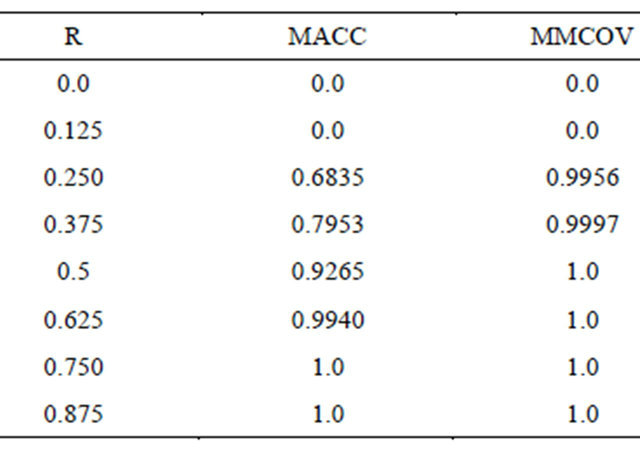
Table 11. Accuracies of strategies A, B, C, D. 10-fold CV; Pima Indians; exhaustive algorithm; r = radius, macc X = mean accuracy of strategy X for X = A, B, C, D.
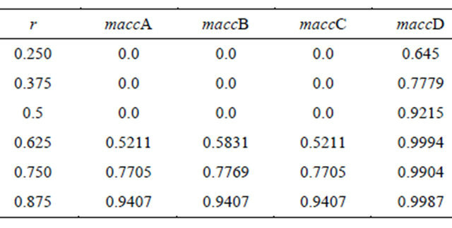
on. Strategy D gives results slightly better than C with the same radii. We conclude that the essential for results of classification is the strategy of treating the missing value of * as * = * in both strategies C and D; the repairing strategy has almost no effect: C and D differ very slightly with respect to this strategy.
5.4. Granular Rough Mereological Classifiers Using Residuals
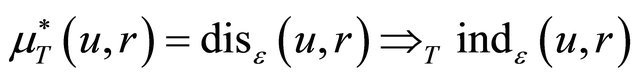
Rough inclusions used in Sections 5.1 - 5.3 in order to build classifiers do take, to a certain degree, into account the distribution of values of attributes among objects, by means of the parameters ε and . The idea that metrics used in classifier construction should depend locally on the training set is, e.g., present in classifiers based on the idea of nearest neighbor, see, e.g., a survey [7]. In order to construct a measure of similarity based on distribution of attribute values among objects, we resort to residual implications-induced rough inclusions. These rough inclusions can be transferred to the universe $ of a decision system; to this end, first, for given objects u, v, and ε in [0,1], factors are defined
 (41)
(41)
and
 (42)
(42)
The weak variant of the rough inclusion  is defined, see [8] and [30-32], as
  if and only if 1.1.15.
 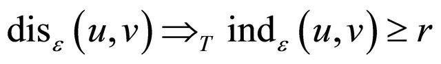 (43)
(43)
These similarity measures will be applied in building granules. Tests are done with the Australian credit data set; the results are validated by means of the 5-fold cross validation (CV-5). For each of t-norms: M, P, L, three cases of granulation are considered:
1) Granules of training objects (GT);
2) Granules of rules induced from the training set (GRT);
3) Granules of granular objects induced from the training set (GGT).
In this approach, training objects are made into granules for a given ε. Objects in each granule g about a test object u, vote for decision value at u as follows: for each decision class c, the value 1.1.16. 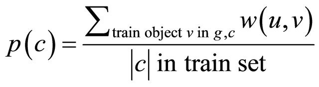 (44)
(44)
is computed where the weight 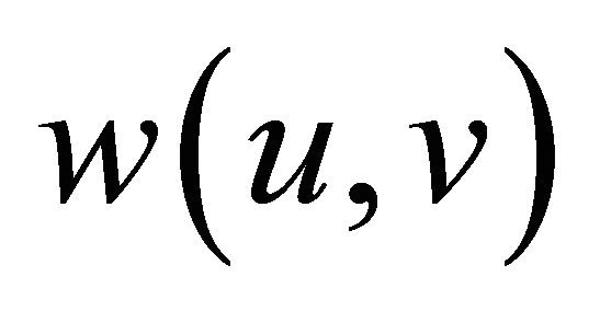 is computed for a given t-norm T as 1.1.17.
 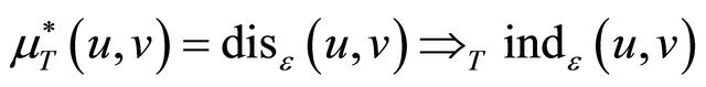 (45)
(45)
The class c* assigned to u is the one with the largest value of p. Weighted voting of rules in a given granule g for decision at test object u goes according to the formula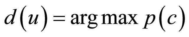 , where 1.1.18.
 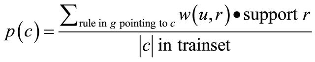 (46)
(46)
and weight  is computed as
 (47)
(47)
The optimal (best) results in terms of accuracy of classification are collected in Table 12.
These results show that rough mereological granulation provides better or at least on par with best results by
Table 12. 5-fold CV; Australian; residual metrics. Met = method of granulation, T = t-norm, ε(opt) = optimal ε, macc = mean accuracy, mean coverage = 1.0 omitted, meanMI = mMI.
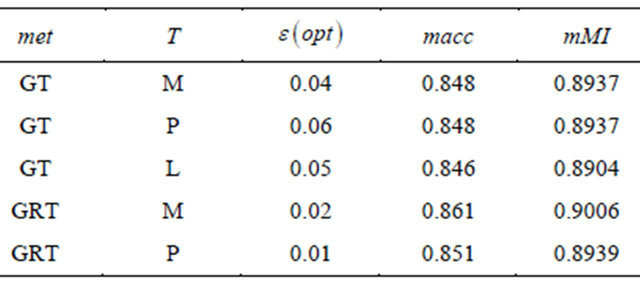
other methods accuracy of classification at the radically smaller classifier size measured as the number of decision rules in it.
5.5. Granular Classifiers: Concept-Dependent and Layered Granulation
In [35], two modifications to the idea of a granular classifier were proposed, viz., the concept-dependent granulation and the layered granulation as well as the hybrid approach merging the two. In concept-dependent granulation, granules are computed as restricted to decision classes of their centers, whereas in layered granulation, the granulation procedure is iterated until stabilization of granules. The experiments with the concept-dependent granulation, for the Australian Credit data set, see [35], Table 3, give, e.g., for the radius r = 0.571429, the accuracy of 0.8865 at the rule set of 2024.4 rules on the average as compared to 12025.0 on the average for nongranular classifier and the size of the training set of granules of 175.5 on the average of granules as compared to the 690 objects in the non-granular case. In the case of layered granulation for the same data set, for, e.g., the granulation radius of r = 0.642857, after four iterations, the accuracy was 0.890, at the number of rules 3275, and, training granule set of size 214.
6. Granular Logics: Reasoning in Information Systems
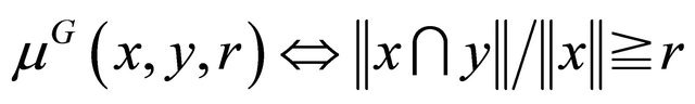
The idea of a granular rough mereological logic consists in measuring the meaning of a unary predicate in the model which is a universe of an information system against a granule defined by means of a rough inclusion. The result can be regarded as the degree of truth (the logical value) of the predicate with respect to the given granule. The obtained logics are intensional as they can be regarded as mappings from the set of granules (possible worlds) to the set of logical values in the interval [0,1], the value at a given granule regarded as the extension at that granule of the intension. For an information/decision system , with a rough inclusion ν, e.g.,
  , on subsets of U and for a collection of unary predicates Pr, interpreted in the universe U (meaning that for each predicate Ф in Pr the meaning [Ф] is a subset of U), we define the intensional logic
  by assigning to each predicate Ф in Pr its intension
  defined by its extension at each particular granule g, as 1.1.19.
 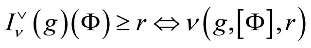 (48)
(48)
With respect to the rough inclusion  the formula (47) becomes
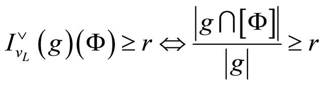 (49)
(49)
A formula Ф interpreted in the universe U of a system  is true at a granule g with respect to a rough inclusion ν if and only if 1.1.20.
  (50)
(50)
and Ф is true if and only if it is true at each granule g. A rough inclusion ν is regular when  holds if and only if
 . Hence, for a regular ν, a formula Ф is true if and only if
  for each granule g. A particularly important case of a formula is that of decision rules; clearly, for a decision rule
  in the descriptor logic, the rule r is true at a granule g with respect to a regular rough inclusion ν if and only if
 (51)
(51)
Analysis of decision rules in the system  can be given in a more general setting of dependencies. For two sets
  of attributes, one says that D depends functionally on C when
 , symbolically denoted C⥟D, where
  is the Xindiscernibility relation defined as, see [10]1.1.21.
  (52)
(52)
Functional dependence can be represented locally by means of functional dependency rules of the form 1.1.22. 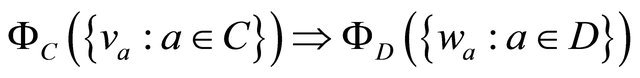 (53)
(53)
where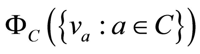 is the formula
 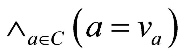 and
and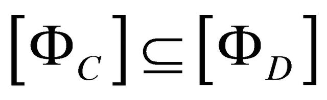 . We introduce a regular rough inclusion on sets
  defined as
 , where r = 1 if
 ,
,  if
if , otherwise r = 0.
Then one proves that  is a functional dependency rule if and only if α is true in the logic induced by
 , see [8]. A specialization of this statement holds for decision rules. Further applications to modalities in decision systems and the Perception Calculus in the sense of Zadeh can be found in [8].
7. Conclusion
We have presented a survey of recent results on rough mereological approach to knowledge discovery. Presented have been applications to problems of data mining (in the form of granular classifiers), intelligent robotics, in the form of mereological potential field based planners, and, a theory of robot formations based on rough mereogeometry. Finally, we have outlined the intensional rough mereological logic for reasoning about knowledge in information/decision systems. These results show that rough mereology can be a valuable tool in the arsenal of artificial intelligence. Results on classification show that granular mereological preprocessing reduces the size of classifiers at as good quality of classification as best obtained in the past by other methods. Formations of autonomous mobile robots defined by means of mereogeometry allow for flexible managing of environments, as shown in respective figures, due to relational character of that definition. Mereological potential fields also deserve an attention due to simplicity of their definition and close geometric relation to the location of the goal and obstacles. We do hope that this survey will give researchers in the fields of Knowledge Discovery and related ones an insight into this new paradigm and will prompt them to investigate it and apply it on their own. There are many problems to investigate, among them, it seems, one of most interesting is whether it is possible to, at least approximately, predict optimal values of parameters of granular classifiers, i.e., of the radius of granulation, the parameter ε, and the catch radius. It this happens, the goal of this survey is achieved.
8. Acknowledgements
The author wishes to thank his former students, Dr Piotr Artiemjew and Paul Osmialowski who cooperated with the author in the tasks of implementing author’s ideas and test them on real data and autonomous mobile robots, respectively.
REFERENCES
- D. Bjoerner, “A Role for Mereology in Domain Science and Engineering,” In: C. Calosi and P. Graziani, Eds., Mereology and the Sciences, Springer Verlag, Berlin, in Press.
- C. Calosi and P. Graziani, “Mereology and the Sciences,” Springer Verlag, Berlin, in Press.
- L. Polkowski, “Mereology in Engineering and Computer Science,” In: C. Calosi and P. Graziani, Eds., Mereology and the Sciences, Springer Verlag, Berlin, in Press.
- L. Polkowski, “Granulation of Knowledge in Decision Systems: The Approach Based on Rough Inclusions. The Method and its Applications,” Proceedings RSEISP 07, Rough Sets and Intelligent Systems Paradigms, Lecture Notes in Artificial Intelligence 4585, Springer Verlag, Berlin, 2007, pp. 271-279.
- L. Polkowski, “A Unified Approach to Granulation of Knowledge and Granular Computing Based on Rough Merology: A Survey,” In: W. Pedrycz, A. Skowron and V. Kreinovich, Eds., Handbook of Granular Computing, John Wiley & Sons, Ltd., Chichester, 2008, pp. 375-400. doi:10.1002/9780470724163.ch16
- L. Polkowski, “Granulation of Knowledge: Similarity Based Approach in Information and Decision Systems,” In: R. A. Meyers, Ed., Encyclopedia of Complexity and System Sciences, Springer Verlag, Berlin, 2009, Article ID: 00788.
- L. Polkowski, “Data Mining and Knowledge Discovery: Case Based Reasoning, Nearest Neighbor and Rough Sets,” In: R. A. Meyers, Ed., Encyclopedia of Complexity and System Sciences, Springer Verlag, Berlin, 2009, Article ID: 00391.
- L. Polkowski, “Approximate Reasoning by Parts. An Introduction to Rough Mereology,” Springer Verlag, Berlin, 2011.
- P. Hajek, “Metamathematics of Fuzzy Logic,” Kluwer Academic Publishers, Dordrecht, 1998. doi:10.1007/978-94-011-5300-3
- Z. Pawlak, “Rough Sets: Theoretical Aspects of Reasoning about Data,” Kluwer, Dordrecht, 1991.
- R. R. Kelly Jr. and C. G. Cegielski, “Introduction to Information Systems: Support and Transforming Business,” 4th Edition, John Wiley & Sons, Ltd., Hoboken, 2012.
- S. Li, T. Li and C. Luo, “A Multi-Granulation Model under Dominance-Based Rough Set Approach,” Lecture Notes in Computer Science, Vol. 7413, Springer Verlag, Berlin, 2012, pp. 18-25.
- B. Liu, Y. Li and Y.-C. Tian, “Discovering Novel Knowledge Using Granule Mining,” Lecture Notes in Computer Science, Vol. 7413, Springer Verlag, Berlin, 2012, pp. 380-387.
- L. Polkowski and P. Osmialowski, “A Framework for Multi-Agent Mobile Robotics: Spatial Reasoning Based on Rough Mereology in Player/Stage System,” Lecture Notes in Artificial Intelligence, Vol. 5306, Springer Verlag, Berlin, 2008, pp. 142-149.
- L. Polkowski and P. Osmialowski, “Navigation for Mobile Autonomous Robots and their Formations: An Application of Spatial Reasoning Induced from Rough Mereological Geometry,” In: A Barrera, Ed., Mobile Robots Navigation, InTech, Zagreb, 2010, pp. 329-354. doi:10.5772/8987
- J. Van Benthem, “The Logic of Time,” Reidel, Dordrecht, 1983.
- H. Choset, K. M. Lynch, S. Hutchinson, G. Kantor, W. Burgard, L. E. Kavraki and S. Thrun, “Principles of Robot Motion. Theory, Algorithms and Implementations,” MIT Press, Cambridge, 2005.
- P. Osmialowski, “On Path Planning for Mobile Robots: Introducing the Mereological Potential Field Method in the Framework of Mereological Spatial Reasoning,” Journal of Automation, Mobile Robotics and Intelligent Systems (JAMRIS), Vol. 3, No. 2, 2009, pp. 24-33.
- P. Osmialowski, “Planning and Navigation for Mobile Autonomous Robots,” PJIIT Publishers, Warszawa, 2011.
- P. Osmialowski and L. Polkowski, “Spatial Reasoning Based on Rough Mereology: Path Planning Problem for Autonomous Mobile Robots,” Transactions on Rough Sets, Vol. 12, Lecture Notes in Computer Science, Vol. 6190, Springer Verlag, Berlin, 2009, pp. 143-169.
- R. Michalski, “Pattern Recognition as Rule-Guided Inductive Inference,” IEEE Transactions on Pattern Analysis and Machine Intelligence PAMI, Vol. 2, No. 4, 1990, pp. 349-361. doi:10.1109/TPAMI.1980.4767034
- L. Polkowski, “Formal Granular Calculi Based on Rough Inclusions (a Feature Talk),” Proceedings of IEEE 2005 Conference on Granular Computing GrC05, Beijing, 25-27 July 2005, pp. 57-62.
- L. Polkowski, “A Model of Granular Computing with Applications (a Feature Talk),” Proceedings of IEEE 2006 Conference on Granular Computing GrC06, Atlanta, 10-12 May 2006, pp. 9-16.
- J. W. Grzymala-Busse, “Mining Numerical Data—A Rough Set Approach,” Transactions on Rough Sets, Vol. 11, Lecture Notes in Computer Science, Vol. 5946, Springer Verlag, Berlin, 2010, pp. 1-14.
- J. G. Bazan, “A Comparison of Dynamic and Non-Dynamic Rough Set Methods for Extracting Laws from Decision Tables,” In: L. Polkowski and A. Skowron, Eds., Rough Sets in Knowledge Discovery, Vol. 1, Physica Verlag, Heidelberg, 1998, pp. 321-365.
- N. S. Hoa, “Regularity Analysis and Its Applications in Data Mining,” In: L. Polkowski, S. Tsumoto and T. Y. Lin, Eds., Rough Set Methods and Applications. New Developments in Knowledge Discovery in Information Systems, Physica Verlag, Heidelberg, 2000, pp. 289-378.
- J. Wroblewski, “Adaptive Aspects of Combining Approximation Spaces,” In: S. K. Pal, L. Polkowski and A. Skowron, Eds., Rough Neural Computing. Techniques for Computing with Words, Springer Verlag, Berlin, 2004, pp. 139-156. doi:10.1007/978-3-642-18859-6_6
- “Rough Set Exploration System (RSES),” http://logic.mimuw.edu.pl/~rses/
- P. Artiemjew, “A Review of the Knowledge Granulation Methods: Discrete vs. Continuous Algorithms,” In: A. Skowron and Z. Suraj, Eds., Rough Sets and Intelligent Systems— Professor Zdzislaw Pawlak in Memoriam, Springer Verlag, Berlin, 2012, pp. 41-59.
- L. Polkowski and P. Artiemjew, “A Study in Granular Computing: On Classifiers Induced from Granular Reflections of Data,” Transactions on Rough Sets, Vol. 9, Lecture Notes in Computer Science, Vol. 5390, 2009, pp. 230-263. doi:10.1007/978-3-540-89876-4_14
- L. Polkowski and P. Artiemjew, “On Classifying Mappings Induced by Granular Structures,” Transactions on Rough Sets, Vol. 9, Lecture Notes in Computer Science, Vol. 5390, 2009, pp. 264-286.
- L. Polkowski and P. Artiemjew, “On Knowledge Granulation and Applications to Classifier Induction in the Framework of Rough Mereology,” International Journal of Computational Intelligence Systems (IJCIS), Vol. 2-4, 2009, pp. 315-331. doi:10.2991/ijcis.2009.2.4.1
- J. W. Grzymala-Busse and Ming Hu, “A Comparison of Several Approaches to Missing Attribute Values in Data Mining,” Lecture Notes in Artificial Intelligence, Vol. 2005, Springer Verlag, Berlin, 2000, pp. 378-385.
- L. Polkowski and P. Artiemjew, “On Granular Rough Computing with Missing Values,” Lecture Notes in Artificial Intelligence, Vol. 4585, Springer Verlag, Berlin, 2007, pp. 271-279.
- P. Artiemjew, “Classifiers from Granulated Data Sets: Concept Dependent and Layered Granulation,” Proceedings RSKD’07 Rough Sets and Knowledge Discovery. Workshop at ECML/PKDD’07, Warszawa, 17-21 September 2007, pp. 1-9.