Open Journal of Modern Hydrology
Vol.06 No.04(2016), Article ID:71689,10 pages
10.4236/ojmh.2016.64020
Quantitative Models to Study the Soil Porosity as Function of Soil Resistivity
M. Juandi
Department of Physics Math and Science Faculty, University of Riau, Pekanbaru, Indonesia

Copyright © 2016 by author and Scientific Research Publishing Inc.
This work is licensed under the Creative Commons Attribution International License (CC BY 4.0).
http://creativecommons.org/licenses/by/4.0/


Received: September 28, 2016; Accepted: October 28, 2016; Published: October 31, 2016
ABSTRACT
Soil degradation is a phenomenon of land subsidence caused by humans. The purpose of this study was to determine the quantitative models of soil porosity. The method used in this research was to measure ground resistance, and determine the value of soil resistivity. Soil porosity was determined by determining the value of the soil volume weight, density of particles, subsequently determined porosity value of land. Based on the research, it has been found quantitative models for the relationship between soil porosity and soil resistivity.
Keywords:
Porosity, Resistivity, Soil

1. Introduction
Soil porosity is one factor that is very important to determine the level of soil fertility, due to the porosity factor influenced by organic matter content, soil structure and soil texture [1] .
The measuring method of soil porosity is commonly performed by a destructive way. This method damages the sample, needs a high cost, and requires a long enough observation time [2] . Determination of porosity by not damaging the sample becomes very necessary; one way is to determine the quantitative relationship between the porosity of the soil and soil resistivity [3] .
Soil resistivity as physical parameter which can be determined by means of an electric current in a soil sample can then be determined the soil resistivity [4] . The pattern of distribution of physical parameters such as soil resistivity and porosity can be used to illustrate the quality of the land around the campus of the Riau University at Tampan District in Pekanbaru City, Riau Province. This mapping is very important because it can be used as data for controlling plant growth and protecting the environment of the University of Riau. Based on the matters mentioned above, it would need to do research on the ground in the area of the University Campus Riau, Tampan District at Pekanbaru.
The purpose of this study is to determine the quantitative model of the relationship between soil porosity and the soil resistivity. The quantitative model can be used to determine the porosity values in the campus area by measuring resistivity values of the University Campus Riau, Tampan District at Pekanbaru.
2. Theory
When two Elekrtroda currents created by a certain distance, such as Figure 1, the potential at the points near the surface will be influenced by both the current electrodes.
Since the flow on both an equal and opposite electrode, the potential at the point P2 as a result of the current electrode C2 can be written:
 (1)
(1)
so that the potential at point P1 due to the current electrode C1 and C2 are:
 (2)
(2)
Using the same way, as is shown in the Figure 2, the potential at P2 due to the current electrode C1 and C2 is,
 (3)
(3)
Finally the potential difference between P1 and P2 can be written as follows:
 (4)
(4)
Of the magnitude of current and potential difference measured the resistivity value can be calculated using the following equation:
 (5)
(5)

Figure 1. Two pairs of current and potential electrodes on the surface of a homogeneous isotropic medium with resistivity ρ [7] .
where k is a geometry factor depending on the placement of electrodes on the surface.
Figure 3 shows the electrodes used in research with geometry factors with a value of k [7] : where in AB/2 = y and MN/2 = x, for , then
 (6)
(6)
In studying the methods of resistivity, should be addressed first electrical laws and regulations. One of the properties that occurred between 2 pieces of electric charge is the charge interactions. The magnitude of the interaction force between two electrical charges have been investigated by Charles Augustin de Coloumb produce:
 (7)
(7)
with is a force vector Coloumb, is the charge source, is the test charge q, r is the distance between the two charges, and is a constant permittivity of vacuum . Now the test charge q is put back into the room, then it will be working a style called Coloumb style, and this situation is said that the room has an electric field Q, The electric field generated by the charge source is:
 (8)
(8)

Figure 2. The pattern of current flow and equipotential field between two electrodes with opposite polarity current [7] .

Figure 3. Electrodes arrangement of geo-electric resistivity survey [7] .
The electric field is a vector quantity whose magnitude can be calculated from the equation, whereas if the charge Q positive direction then the direction of the electric field leave the source, when the opposite charge Q source is negative then the electric field direction toward the source. Electric potential energy of a charge is defined as the effort required toremove the charge from infinity to the point charge is located.
 (9)
(9)
while the electric potential (V) itself is defined as the potential energy of unity test charge.
 (10)
(10)
Ohm’s law illustrates the relationship between the amount of electric potential (V), a strong current (I) and the amount of resistivity or conductive R is written as follows:
 (11)
(11)
now review the relationship between the current density, electric field and the electric potential in the scalar notation thus:

 (12)
(12)
and the current density values obtained as follows:
 (13)
(13)
Magnitude is a scale that indicates the characteristics of a conducting material. This quantity is a scalar quantity which is commonly referred to as the electrical con- ductivity of the material by the following equation:
 (14)
(14)
The unit is the I/Ohm∙meter. The opposite of resistivity or conductivity is commonly called the resistivity material by the equation:
 (15)
(15)
or,
 (16)
(16)
Based on Ohm’s law, the relationship between the electric current density, the electric field and the conductivity of the medium which is expressed in the following equation:
 (17)
(17)
for the electric field is a conservative field, it can be expressed in terms of potential gradient as follows:
 (18)
(18)
if there is no source of the charge accumulated in the regional area,
 (19)
(19)
for homogeneous isotropic medium, then it is a scalar constant vector in space, so that the Equation (19) becomes:
 (20)
(20)
because of the symmetry of the ball, potential only as a function of distance r from the source, then obtained the following equation:
 (21)
(21)
Completion of these equations can be integral or differential equations. By integrating the two times we get,
 (22)
(22)
where A and B integral constants whose values depend on the boundary conditions, therefore V = 0 in the obtained B = 0, so the electric potential has a value inversely proportional to the distance from the source point .
.
Properties of electricity in the soil can be classified into conduction electronically. This conduction occurs when rocks or minerals have many free electrons that electric current circulate in rocks or minerals by the free electrons. The flow of electricity is also influenced by the nature or characteristics of each rock that passed him. One of the properties or characteristics of the rock is the resistivity (resistivity) that indicates the material’s ability to conduct electricity. The greater the value of the resistivity of a material, the more difficult these materials conduct electricity and vice versa. The resistivity has a different understanding with the resistance (resistance), wherein the resistance does not only depend on the material, but also depends on factors geometry or shape of the material, while the resistivity does not depend on the geometry factor. If the terms of a cylinder of length L, cross-sectional area A and resistance R, the following equation obtained by Figure 4.
Physically these formulas can be interpreted if the length of the cylinder conductor (L) is raised, then the resistance will increase and if the diameter of the conductor lowered the mean cross-sectional area (A) is reduced, the resistance also increases. Where is the resistivity (resistivity) in ohm.m, while according to Ohm’s law, resistivity formulated [5] :
 (23)
(23)

Figure 4. Cylindrical conductor.
3. Method
The method used in this study is an experimental method, Tools and materials used in this research that GPS, container, soil samples, ring samples, oven, eksikator, digital scales, measuringcups, meters, pipes, calipers, battery, ammeters, voltmeters, cables, devices surfer, microsoft excel and laptops.
The first thing done is to determine the coordinates of the point of use GPS, then do the soil sampling at a depth of 20 cm. Samples have been taken from several locations then measured levels of resistivity and porosity levels are calculated.
Measurement procedure porosity of the soil: weigh empty tube, for example weighs Y grams, put the tube in an upright position standing on the soil surface to be measured heavy volume of soil, press the tube slowlyso that all the tubes into the ground, lift the jar with soil, then wipe the dirt on the side of the tube outer, smooth surface of the soil to the surface of both ends of the ring samples, then cover both ends of the ring with a lid, ring were taken to the laboratory, then dry in the oven with a temperature of 105˚C, until its weight is constant, weigh the tube and its contents her, for example, X-gram weight, remove the soil in the ring and calculate the dry weight of the soil by reducing X with Y, Z grams weighs example, calculate the volume of soil or equal to the volume of soil, e.g. A cm3 volume. calculate the volume weight of the soil by the formula: weight of soil volume (ρb) = Z/A g/cm3, determine the moisture content of air-dry soil to be used or the use of dry soil absolute., weigh vinometer/pumpkin Erlenmeyer, weigh 50 grams of dry soil absolute, and then inserted into vinometer/pumpkin Erlenmeyer 100 ml, fill vinometer with water load ion or distilled water while rinsing ground attached to the neck pumpkin until half-filled pumpkins, education vinometer slowly a few minutes, occasionally pumpkin shaken carefully to prevent the loss of soil along the foam, cool the flask and its contents until it reaches room temperature, then add distilled water cooler that has been boiled prior to the limit volume, cap and clean the outside of the pumpkin with a dry cloth, and its contents weighed vinometer, for example, weighs Z grams [6] .
 (24)
(24)
 (25)
(25)
Density of water = 1, then the weight of water equal to the volume of water, calculate the volume of the soil by reducing the volume of the flask with a volume of water (A). Calculate the density of particles with the formula: density of particles:
 (26)
(26)
Porosity is calculated using Equation (27).
 (27)
(27)
4. Result and Discussion
Based on the correlation test soil samples Region University of Riau carried out in twelve points, namely, Faculty of Engineering, Faculty of Agriculture, Faculty of Fisheries, the Main Stadium, Stadium Mini, Rector UR, Rock Climbing, Natural Sciences, FEKON, FISIP, FKIP, RS UR obtained a quantitative relationship between porosity soil resistivity i.e.: Φ = 66,443ρ−2.068 where (Φ) is the porosity and (ρ) is resistivity, with a correlation of 0.919, meaning that there is a strong relationship between the resistivity with the porosity, as shown in Figure 5.
Figure 5 looks the empirical relationship between porosity and resistivity in which the figure shows the relationship of porosity and soil resistivity inversely, the greater the porosity the less resistivity.
For the purpose of mapping the resistivity values measured as much as 400 points in the campus of the University of Riau, further mapping resistivity values in the area of the campus of the University of Riau as shown in Figure 6. Based on the distribution of resistivity values were obtained from 26 ohm∙m up to 44 ohm∙m, it can be said that the type of soil area of the campus of University of Riau nearly homogeneous.
From the field observations that the pores in the samples can be occupied by water, causing the value of the resistivity becomes small, generally dominated for a region still closed with trees, thus increasing the attraction between water with soil particles.
Figure 6 shows the resistivity contours of the soil, shows the distribution of the resistivity profile cross section of North-South, and shows the distribution of the resistivity profile cross section West-East. Each is shown in Figure 7 and Figure 8.
The cross-section from north to south shows the trend rate of resistivity decreases, but the area around 0.0005 folder units to 0.002 units reversal of the direction, that the value

Figure 5. Quantitative models of soil porosity as function of soil resistivity.

Figure 6. Contour soil resistivity level of 400 points in the campus of the University of Riau.
of resistivity starts to rise. From west to east cross section showing the same tendency resistivity level, but had been a reversal, where the resistivity values rise and fall in some areas such as around 0 to 0.003 map units and an area of 0.008 to 0.009 map units.
Resistivity mapping results in Figure 6 subsequently converted at the rate of porosity by using a quantitative model that was obtained, as shown in Figure 6.
Figure 9 is a contour level of porosity of the soil in the area of the campus of University of Riau in view two-dimensional (2D). Based on Figure 6 and Figure 9, it can be

Figure 7. Soil resistivity distribution profile based on a cross-section of North-South.

Figure 8. Soil resistivity distribution profile based on a cross-section of West-East.

Figure 9. Mapping porosity of the soil based on a quantitative model on the campus of the University of Riau in Pekanbaru City, Riau Province.
said that if a large resistivity, the porosity will be small. The highest soil porosity percentage found in the area of the Faculty of Economics is 63.35%, and the lowest soil porosity percentage found in the Main Stadium is 28.66%. To some point which also has a large porosity as FKIP 59.24%, 57.2% FAPERTA, Hospital UR 53.12%, 53.12%, Faculty of Engineering, UR Mini Stadium FAPERIKA 51.08% and 49.04% and several points which also has a small porosity as FMIPA 38.85%, FISIP 47.01% and Recto rate 40.89%. Figure 10 shows distribution of soil porosity in the North-South cross-section, and Figure 11 shows that of the West-East cross section.
Figure 10 and Figure 11 are a cross-sectional profile to US soil porosity and BT. The cross-section from north to south shows the trend level of porosity is increased, but the area around 0.0005 folder units to 0.002 units reversal direction, i.e. porosity values began to fall. From west to east cross section showing the same tendency porosity level, but had been a reversal in some areas, where porosity values fell on the area around 0 to 0.001 map units, map units 0.002 to 0.0025, 0.008 to 0.009 map units and rises high enough in the area of about 0.001 to 0.002 map units. Results grouping level of soil

Figure 10. Soil porosity distribution profile based on cross-section of North-South.
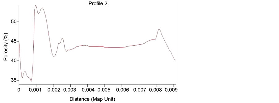
Figure 11. Soil porosity distribution profile based on cross-section of West-East.

Table 1. Results grouping level of soil quality in the campus of the University of Riau based on quantitative model of the resistivity porosity.
quality in the area of Riau University Campus based quantitative models porosity can be seen in Table 1.
5. Conclusion
Based on the research that has been done, some conclusions can be drawn as follows: 1) Quantitative Models of the Soil Porosity as Function of Soil Resistivity are formulated as Φ = 66.443ρ−2.068, where (Φ) is the porosity and (ρ) is resistivity, with a correlation of 0.919, meaning that there is a strong relationship between the resistivity and the porosity; 2) The spread of soil resistivity distribution in the area of Riau University campus at Tampan District from north to south and from west to east has a tendency to decline, otherwise the distribution of porosity level has a tendency to rise, these results that are in accordance with the quantitative models are obtained.
Cite this paper
Juandi, M. (2016) Quantitative Models to Study the Soil Porosity as Function of Soil Resistivity. Open Journal of Modern Hydrology, 6, 253-262. http://dx.doi.org/10.4236/ojmh.2016.64020
References
- 1. Notohadiprawiro, T. (1998) Soil and Environment. Director General of Higher Education, Jakarta.
- 2. Alfi, A.M. (2011) Report of Practical Fundamentals of Soil Science, Faculty of Agriculture. University of Bengkulu.
- 3. Arsyad, S. (2000) Soil and Water Conservation. Information Resources Bogor Agricultural Institute. IPB Press, Bogor.
- 4. Grant, F.S. and West, G.F. (1965) Interpretation Theory in Applied Geophysics. McGraw-Hill Book Company, New York.
- 5. Halliday, D. and Resnick, R. (1978) Fundamentals of Physics. Cambridge University Press, New York, London.
- 6. Krossblade, L. (1989) Soil and Rock Backfill Compaction by Vibration. DRI Translation Kartasa-Poetra, Bina Literacy, Jakarta, 111.
- 7. Dobrin, M.B. (1981) Introduction to Geophysical Prospecting. McGraw-Hill, New York.