Open Journal of Acoustics
Vol.05 No.04(2015), Article ID:62211,11 pages
10.4236/oja.2015.54016
Analytical Computation of Acoustic Bidirectional Reflectance Distribution Functions
Jaume Durany1, Toni Mateos2, Adan Garriga3
1Department of Information and Communication Technologies, Universitat Pompeu Fabra, Barcelona, Spain
2Dolby Laboratories, Barcelona, Spain
3Eurecat-Technology Centre of Catalonia, Barcelona, Spain

Copyright © 2015 by authors and Scientific Research Publishing Inc.
This work is licensed under the Creative Commons Attribution International License (CC BY).
http://creativecommons.org/licenses/by/4.0/


Received 2 December 2015; accepted 22 December 2015; published 25 December 2015
ABSTRACT
The Room Acoustic Rendering Equation introduced in [1] formalizes a variety of room acoustics modeling algorithms. One key concept in the equation is the Acoustic Bidirectional Reflectance Distribution Function (A-BRDF) which is the term that models sound reflections. In this paper, we present a method to compute analytically the A-BRDF in cases with diffuse reflections parametrized by random variables. As an example, analytical A-BRDFs are obtained for the Vector Based Scattering Model, and are validated against numerical Monte Carlo experiments. The analytical computation of A-BRDFs can be added to a standard acoustic ray tracing engine to obtain valuable data from each ray collision thus reducing significantly the computational cost of generating impulse responses.
Keywords:
Room Acoustics, Room Acoustic Rendering Equation, Vector Based Scattering, Ray Tracing, Audio Rendering

1. Introduction
Computers have been used for over thirty years to model room acoustics. Nowadays, computational acoustics modeling has become a common practice in many different disciplines: the acoustic design of buildings such as auditoria or concert halls [2] [3] , outdoor acoustics [4] , audio post-production in Digital Cinema [5] or audio for video-games and other interactive applications [6] -[8] .
The most used techniques in computational room acoustics are the so-called geometrical methods which are based on the geometrical theory of acoustics [9] . The general approach of the geometrical methods is to find significant paths along which sound can travel from a source to a receiver through the environment. The most important geometrical methods that have been applied to acoustics are: image source method [10] [11] , ray tracing [12] , beam tracing [13] -[15] and radiosity [16] -[18] . Some of these (sometimes in combination) are the basis of many room acoustics commercial softwares such as EASE [19] , Odeon [20] , Catt-Acoustics [21] or Ramsete [22] .
Recently, Siltanen et al. introduce the Room Acoustic Rendering Equation [1] which is a model for acoustic energy propagation. This approach, borrowed from computer graphics, integrates several geometrical methods within the same theoretical framework. One key concept in the equation is the Acoustic Bidirectional Reflectance Distribution Function [23] (A-BRDF) which is the term that models sound reflections.
In the present paper, we develop a method to compute the analytical solution for the A-BRDF in cases where sound reflections are diffuse, and diffusion is parametrized by one (or more) random variables. The method makes use of various properties of continuous probability functions, and exploits the relation between two and three dimensional probability densities.
The method is applied to the Vector Based Scattering Model [24] (VBS), which is one of the existing ways to efficiently include diffusion in a ray tracing algorithm by means of random vectors. Analytical results are obtained and shown to coincide with the large number of rays limit of the corresponding Monte Carlo simulation.
The paper is organized as follows: Section 2 briefly reviews the Room Acoustic Rendering Equation and the application of BRDFs to acoustics. Section 3 introduces the general methodology to compute analytically the A-BRDF. Section 4 presents the analytical computation of the A-BRDF for the Vector Based Scattering Model, and the comparison with the corresponding Monte Carlo results. Finally, future work and conclusions are discussed in Section 5.
2. Acoustic BRDF
Let us briefly review the Room Acoustic Rendering Equation (RARE) introduced in [1] , which models the propagation of acoustic energy through the environment both in diffusive and general non-diffusive conditions. Following the notation in [1] , the RARE reads:
 (1)
(1)
where
 is the set of all surface points in the enclosure,
 is the outgoing time-dependent radiance from point
 in the direction
 ,
,
 is the radiance emitted by the surface from
 in the direction
 , and
, and
 is the reflection kernel where x is the location of the previous reflection. The reflection kernel is a product of three terms:
 (2)
(2)
where
 is the visibility term,
 is the geometry term,
 is the A-BRDF, and
 stands for the direction of the rays. Henceforth, directions will also be specified either using unit-norm vectors or using a specific coordinate system on the sphere,
 , the zenital and azimuthal angles, respectively, as shown in Figure 1.
All the physics of the problem is contained in the A-BRDF, which can be expressed as the following ratio (see Figure 1),
 (3)
(3)
where
 is the radiance at a point
 , exiting along the outgoing direction
 ; and
; and
 is the irradiance at the same point incident along the direction
 . Again, x represents the location of the previous reflection of the sound ray.

Figure 1. The A-BRDF returns the ratio of reflected radiance,
 , to the incident irradiance,
 , at point
 .
.
The A-BRDF can be interpreted as the probability that sound energy incident from a direction
 is reflected in the direction
 .
.
As such, the A-BRDF must also be normalized in order to avoid an artificial increase of the acoustic energy in the system. For the sake of simplicity of notation, in the rest of this paper we will not consider explicit dependence of the A-BRDF on the reflection position , and hence write
 .
.
3. General Methodology
In this section we present a method to compute analytically the A-BRDF in cases where reflections suffer diffusion parameterized by a random variable, i.e. in cases where the vector
 along the outgoing direction,
 , is determined using a random vector,
 ,
,
 (4)
(4)
governed by a probability density . The subindex denotes that
 is a 3-dimensional probability density, i.e.
 yields the differential probability that the vector lies in the interval
 . We have chosen a random vector in
 rather than a single random variable, to cover more general cases, such as the VBS model discussed in the next section. We have also included dependence on the incident direction of the sound ray, represented by the unitary vector
 with direction
 1 (see Figure 2).
To compute the A-BRDF in such cases, we will use Equation (4), which relates the outgoing direction and the random vector , to obtain a relation between the probability density of the outgoing direction, and
 . In other words, we will use Equation (4) to obtain the probability that the outgoing ray is in a small neighborhood
 , which is precisely the information provided by
 .
.
The relation between probability densities can be obtained recalling the way differential forms transform under a change of coordinates,
 (5)
(5)
which yields the following relation
 (6)
(6)
Here,
 is the Jacobian of the transformation defined by Equation (4).
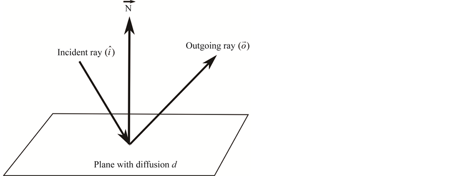
Figure 2. The outgoing ray
 will be function of the incident ray
 and other parameters.
One last step is needed to obtain the A-BRDF. Note that
 contains information about the probability that the outgoing vector
 has modulus
 between
 , besides the probability that it has direction between
 . Thus, to obtain
 , all that is left to do is an integration over all possible moduli:
 (7)
(7)
Note that the need for this last integration arises from the fact that relations of the form (4) are often written in a manner where the outgoing vector is not guaranteed to have unit norm, as will be shown in the next section.
The general method presented here can also apply to cases where the random vector is unitary, which is the case of VBS. In such cases, the probability density of the random unit vector
 is actually two-dimen- sional, and it can be seen as the restriction to the unit sphere of the three-dimensional probability density
 ,
,
 (8)
(8)
where . This relation guarantees that probabilities can be indistinctly computed integrating
 or
or
 over two or three-dimensional intervals, respectively,
 (9)
(9)
4. A-BRDF for the Vector Based Scattering Model
Although several ray tracing simulations propagate rays using only specular reflections, one of the existing choices in room acoustic simulations is to include a diffusion model to determine the direction of the outgoing rays. The Vector Based Scattering (VBS) [24] is a method for room acoustics ray-tracing computations that makes use of a specific model to parameterize diffusion of sound waves by obstacles. Within VBS, the vector along the outgoing ray,
 , is calculated via a linear combination of two vectors
 (10)
(10)
where
 is a unit vector along the specular direction,
 is a random unit vector, and
 is the diffusion coefficient of the material (see Figure 3). Clearly,
 is entirely determined by the incident vector
 , and thus, Equation (10) is an explicit example of the general Equation (4).
In this case, the random vector
 is uniformly distributed along the hemisphere whose equator is the plane of collision, and which contains the incoming and outgoing rays. The problem of determining the outgoing direction can be thought of that of adding a random vector of length d to the outgoing unit vector, after rescaling by
 (see Figure 3).
4.1. Analytic Computation of A-BRDF
In this section, we focus on a slight variation of the VBS model whereby the random vector
 is uniformly distributed along a whole unit sphere, rather than a hemisphere (Figure 4). This variation simplifies the presentation of the computations and allows for a deeper analysis of the results. The extension to the common case of the upper hemisphere, although straightforward, is more cumbersome, and will be presented elsewhere.
To obtain the A-BRDF we need to use Equation (7), which in turn depends on the relation between probability densities in Equation (6). The VBS is an example where the random vector has unit norm, and therefore requires Equation (8),
 (11)
(11)
where , the Dirac
 -term ensures that the random vector is unitary (see Equation (8)), and the choice
 ensures that the probability is normalized to one:
 (12)
(12)
To complete the computation in Equation (6), we need the Jacobian of the transformation (10), which turns out to be constant,
 (13)
(13)

Figure 3. Scheme of the VBS, with
 randomly generated within the upper hemisphere.

Figure 4. Scheme of the VBS, with
 randomly generated within the whole sphere.
To continue, we need to invert Equation (10) and express the modulus
 as a function of the outgoing and incident rays:
 (14)
(14)
where
 is the cosine between the specular and the outgoing directions. Note that expressing
 as a function of
 does not guarantee that
 is unitary; this fact is only ensured by the delta-function in Equation (13). The expression for the probability density of the outgoing vector is then given by:2
 (15)
(15)
The last step to obtain the A-BRDF consists on inserting Equation (15) in Equation (7) and integrating over the radial coordinate. From (15), it is clear that, in this case, the A-BRDF depends on the incident and outgoing directions only through the combination . We shall thus write
 in the remainder of the paper. From (7):
 (16)
(16)
This integral is straightforward using a general formula for integrals containing Dirac’s delta functions:
 (17)
(17)
where the sum is over all roots
 of the function
 in the interval
 . In our case,
 has at most two roots,
 :
:
 (18)
(18)
Each of these roots contributes to the integral in Equation (16) only when they are real and positive, the latter restriction due to the fact that the integral range is . Thus, given that
 , depending on the value of
 we obtain one of the following results
 (19)
(19)
The condition that both solutions be real is
 (20)
(20)
which basically states that unless diffusion is high enough, there are outgoing angles that are unattainable for some incident directions. Indeed, it can be seen that Equation (20) is always satisfied if
 (all directions attainable), and not satisfied for some outgoing directions if
 (presence of unattainable directions).
Similarly, only
 is positive if
 , which yields
 (21)
(21)
whereas both
 and
and
 are positive if
 , which yields
 (22)
(22)
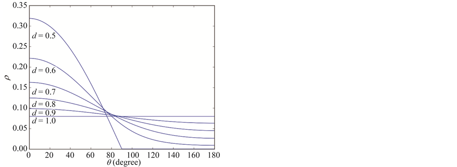
Figure 5 shows various plots of the analytical results for the A-BRDF, Equations (21) and (22). The two extreme limits work as expected: when , all outgoing directions are equally probable (Lambert diffusion limit); whereas when
 , only outgoing directions close to specularity (
 ) are attainable.
The results for
 are also intuitive: the probability density of the outgoing ray is maximum at specularity, and decreases progressively away from it. The maximum is less pronounced as we increase the diffusion coefficient attaining a uniform distribution for
 .
.
The results for
 might look anti-intuitive at first sight. Besides the existence of a limit angle
 explained above, it is worth remarking that the maximum of the probability density does not lie at specularity, but very close to the limit angle. Indeed, the probability density diverges at
 . As shown in the next section, this divergence is actually integrable, and therefore leads to finite and meaningful measurable probabilities. To understand physical origin of this divergence note that, when
 , the outgoing vector
 lies on the sphere centered at
 , as shown in Figure 3. The limit angle corresponds to a line with origin at the reflection point, and which is tangent to the sphere. The probability density that
 lies in the interval
 is basically the fraction of area of the sphere that lies between those two angles. At strict tangency, no matter how small
 , there is always a finite area lying in the range.3
4.2. Analysis and Numerical Validation
In this section we will validate Equations (21) and (22) by showing that Monte Carlo experiments reproduce the same results in the limit of large number of rays. To avoid subtleties with the divergences explained above, we will compare probability distributions rather than probability densities; the former contains the same information as the latter, but it is necessarily absent of divergences.
The probability of having an outgoing ray contained in a finite solid angle
 can be obtained from the probability density via
 (23)
(23)
Given that, as described above,
 depends only on the cosine angle
 , we will compare with Monte Carlo experiments the probability
 that the outgoing ray has an angle
 with respect to the
 (a) (b)
Figure 5. Analytical results of the A-BRDF for diffusion values larger (a) and lower (b) than 1/2.
specular direction less than , irrespective of the rotational angle
 ,
,
 (24)
(24)
Our analytical prediction for
 follows from (21) and (22):
 (25)
(25)
where , and
, and
 is the indefinite integral of
 , which can be computed analytically. For
 ,
,
 (26)
(26)
whereas for ,
,
 (27)
(27)
We will now show that Equations (26) and (27) provide same result as Monte Carlo experiments in the limit of large number of rays. In order to do so, consider a single plane characterized by a diffusion coefficient d. To simplify the experiment, let us set the direction of the incident sound ray to be orthogonal to the plane, which leads to a specular vector,
 , that coincides with the normal to the plane. For a given value of the diffusion coefficient, N random 3-vectors
 ,
,
 are produced and added to the specular vector following the VBS Equation (10), thus obtaining N outgoing rays
 .
.
Figure 6 shows the histogram (red points) corresponding to the outgoing directions of the vectors
 and its comparison to the analytical results (blue continuous lines). A large number of random rays
 was used. The agreement is excellent.
The usefulness of the analytic results presented here is more apparent when the convergence of the Monte Carlo results is considered. Figure 7 shows a set of plots for fixed diffusion
 and varying number of random rays:
 . These plots can be used to estimate the needed number of rays that would be needed, if analytical results were not available, to fulfill each particular ray-tracing precision criteria.
4.3. Use of Analytical A-BRDFs in Acoustic Ray Tracing Engines
Acoustic ray tracing enginges find propagation paths between a source and receiver by generating rays emanating from the source position and following them through the environment until a set of rays reach the receiver [12] . The final objective is to make use of the rays that reach the receiver to obtain the Impulse Response that characterizes the acoustic field of the room.
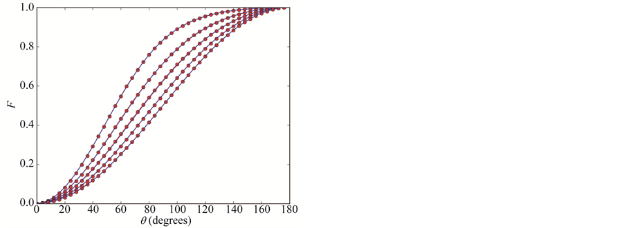

Figure 6. Analytic curves (blue lines) for the distribution function compared to Monte Carlo results (red dots) based on
 random rays, for
 (left), and
 (right).


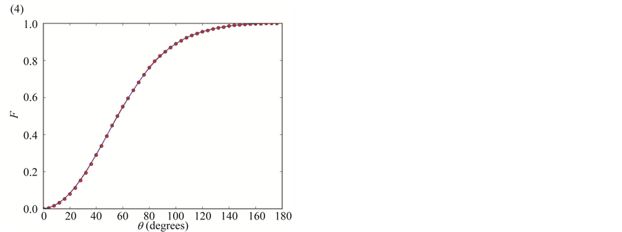
Figure 7. Analytic curves (blue lines) compared to Monte Carlo results (red dots), for
 and different number of random rays:
 (1),
(1),
 (2),
(2),
 (3) and
 (4).
(4).
A large number of rays is needed in order to obtain accurated results. For instance, AURA module included in EASE acoustic simulator software generates around 105 rays for medium size rooms [25] . The computation of analytical solutions for the A-BRDF can be added to a standard acoustic ray tracing engine in order to reduce significantly the amount of rays needed to obtain the same results. The proposed methodology provides valuable data at each collision for all the rays that are generated and followed through the enclosure.
The resulting ray tracing algorithm incorporates an extra step every time a ray collides with the environment. In addition to compute the outgoing ray direction, it makes use of the analytical solution for the A-BRDF to compute the contribution of the collision to the final Impulse Response.
Figure 7 shows that the analytical solution of the A-BRDF gives the same result that can be obtained by throwing a large number of rays (104 rays were needed in our plots to match the analytical solution). Accordingly, the addition of the anaylical solution to the ray tracing algorithm notably reduces the amount of rays needed to obtain the same accuracy in the resulting Impulse Responses.
5. Conclusions
A method to derive analytical solutions for the Acoustic Bidirectional Reflectance Distribution Function (A-BRDF) in cases of diffuse reflections parametrized by random variables has been presented and discussed. The method works for generic relations between outgoing, incoming and random vectors of the form (4), and makes use of various properties of continuous probability functions, exploiting the relation between two and three dimensional probability densities.
The method has been applied to the well-known Vector Based Scattering Model, for which exact analytical A-BRDF has been obtained, Equations (21) and (22). The results provide, by means of only one analytical formula evaluation, the same results as the corresponding Monte Carlo simulation in the limit of large number of rays.
The computation of analytical solutions for the A-BRDF can be added to a standard acoustic ray tracing engine by introducing an extra step in the algorithm to compute the contribution of every ray collision with the environment to the final Impulse Response. That is, instead of only using the information coming from the rays that reach the listener position to compute the Impulse Response, valuable data can be obtained from each collision that contributes to the computation of the Impulse Response thus reducing significantly the computational cost, as shown in Figure 7. The use of this methodology can imply a reduction of about 103 - 104 rays in any of the existing comercial acoustic ray tracing engines. Further work will focus on the application of the method discussed here to other ray tracing diffusion models for acoustics and on the computation of real time Impulse Responses for simple environments through the method introduced in this paper.
Acknowledgements
The authors wish to thank Jordi Arqués, Daniel Arteaga, Pau Arumí, Giulio Cengarle, David Garcia, Natanael Olaiz, Ferran Orriols and Carlos Spa for help and discussions.
Cite this paper
JaumeDurany,ToniMateos,AdanGarriga, (2015) Analytical Computation of Acoustic Bidirectional Reflectance Distribution Functions. Open Journal of Acoustics,05,207-217. doi: 10.4236/oja.2015.54016
References
- 1. Siltanen, S., Lokki, T., Kiminki, S. and Savioja, L. (2007) The Room Acoustic Rendering Equation. The Journal of the Acoustical Society of America, 122, 1624-1635.
http://dx.doi.org/10.1121/1.2766781 - 2. Kuttruff, K. (2000) Room Acoustics. Elsevier Science Publisher, New York, 367 p.
- 3. Rindel, J.H. (2000) The Use of Computer Modeling in Room Acoustics. Journal of Vibroengineering, 4, 219-224.
- 4. Salomons, E.M. (2001) Computational Atmospheric Acoustics. Kluwer Academic Publishers, Netherlands, 335 p.
http://dx.doi.org/10.1007/978-94-010-0660-6 - 5. IP-Racine Consortium (2006) Digital Cinema Perspectives. BCM éditions, Belgium, 254 p.
- 6. Funkhouser, T. (2002) Sounds Good to Me! Computational Sound for Graphics, Virtual Reallity and Interactive Systems, SIGGRAPH Course Notes.
- 7. Savioja, L., Huopaniemi, J., Lokki, T. and Väänänen, R. (1999) Creating Interactive Virtual Acoustic Environments. Journal of the Audio Engineering Society, 47, 675-705.
- 8. Savioja, L. (1999) Modeling Techniques for Virtual Acoustics. PhD Thesis, Helsinki University of Technology, Finland.
- 9. Morse, P.M. and Ingard, K.U. (1986) Theoretical Acoustics. Princeton University Press, Princeton.
- 10. Allen, J.B. and Berkley, D.A. (1979) Image Method for Efficiently Simulating Small-Room Acoustics. The Journal of the Acoustical Society of America, 65, 943-950.
http://dx.doi.org/10.1121/1.382599 - 11. Borish, J. (1984) Extension of the Image Model to Arbitrary Polyhedra. The Journal of the Acoustical Society of America, 75, 1827-1836.
http://dx.doi.org/10.1121/1.390983 - 12. Krokstad, A., Strom, S. and Sorsdal, S. (1968) Calculating the Acoustical Room Response by the Use of a Ray Tracing Technique. Journal of Sound and Vibration, 8, 118-125.
http://dx.doi.org/10.1016/0022-460X(68)90198-3 - 13. Funkhouser, T., Tsingos, N., Carlbom, I., Elko, G., Sondhi, M., West, J., Pingali, G., Min, P. and Ngan, A. (2004) A Beam Tracing Method for Interactive Architectural Acoustics. The Journal of the Acoustical Society of America, 115, 739-756.
http://dx.doi.org/10.1121/1.1641020 - 14. Funkhouser, T., Carlbom, I., Elko, G., Pingali, G., Sondhi, M. and West, J. (1998) A Beam Tracing Approach to Acoustic Modeling for Interactive Virtual Environments. SIGGRAPH’98: Proceedings of the 25th Annual Conference on Computer Graphics and Interactive Techniques, New York, 24 July 1998, 21-32.
- 15. Laine, S., Siltanen, S., Lokki, T. and Savioja, L. (2009) Accelerated Beam Tracing Algorithm. Applied Acoustics, 70, 172-181.
http://dx.doi.org/10.1016/j.apacoust.2007.11.011 - 16. Nosal, E.M., Hodgson, M. and Ashdown, I. (2004) Investigation of the Validity of Radiosity for Sound-Field Prediction in Cubic Rooms. The Journal of the Acoustical Society of America, 116, 3505-3514.
http://dx.doi.org/10.1121/1.1811473 - 17. Nosal, E.M., Hodgson, M. and Ashdown, I. (2004) Improved Algorithms and Methods for Room Sound-Field Prediction by Acoustical Radiosity in Arbitrary Polyhedral Rooms. The Journal of the Acoustical Society of America, 116, 970-980.
http://dx.doi.org/10.1121/1.1772400 - 18. Siltanen, S., Lokki, T. and Savioja, L. (2009) Frequency Domain Acoustic Radiance Transfer for Real-Time Auralization. Acta Acustica United with Acustica, 95, 106-117.
http://dx.doi.org/10.3813/AAA.918132 - 19. EASE. http://ease.afmg.eu
- 20. Odeon. http://www.odeon.dk
- 21. CATT-Acoustic. http://www.catt.se
- 22. Ramsete. http://www.ramsete.com
- 23. He, X., Torrance, K., Sillon, F. and Greenberg, D. (1991) A Comprehensive Physical Model for Light Reflection. ACM SIGGRAPH Computer Graphics, 25, 175-186.
http://dx.doi.org/10.1145/127719.122738 - 24. Christensen, C.L. and Rindel, J.H. (2005) A New Scattering Method That Combines Roughness and Diffraction Effects. The Journal of the Acoustical Society of America, 117, 2499.
http://dx.doi.org/10.1121/1.4788035 - 25. AURA Module for EASE. http://ease.afmg.eu/index.php/AURA_Module.html
NOTES
1Note that Lambert diffusion is an extreme case of (4) where the outgoing direction does not depend on the incoming one.
2We have used the equality
 to avoid the use of square roots inside delta-functions.
3A simpler analogous problem is that of finding the fraction of length of the unit circle
 that lies in a small interval
 . The answer diverges at
 despite the fact the total length is, obviously, finite. At those points,
 lines intersect the circle tangentially.