Open Journal of Acoustics
Vol.3 No.3A(2013), Article ID:36864,12 pages DOI:10.4236/oja.2013.33A005
Study of Fourier-Based Velocimetry
1Imperial College London, South Kensington Campus, London, UK
2Department of Medical Physics and Bioengineering, University College London, London, UK
Email: jm.mari@ucl.ac.uk
Copyright © 2013 Jean Martial Mari. This is an open access article distributed under the Creative Commons Attribution License, which permits unrestricted use, distribution, and reproduction in any medium, provided the original work is properly cited.
Received July 18, 2013; revised August 18, 2013; accepted August 25, 2013
Keywords: Doppler; Fourier; Ultrasonic Imaging; Wideband; High Speed
ABSTRACT
Standard phase-domain pulsed Doppler techniques used in Colour Flow Mapping such as spectral Doppler or autocorrelation are monochromatic, focused on the analysis of the centre transmit frequency. As such all the algorithms using those approaches are limited: in terms of spatial Doppler resolution because of the long pulses typically used for transmission, in terms of frame rate because of the necessity to perform many Doppler lines repetitions and additional B-mode imaging transmissions, and in terms of accuracy which depends on the stability of the Doppler signal at the frequency considered. A velocimetry technique is presented which estimates the shifts between successive Doppler line segments using the phase information provided by the Fourier transform. Such an approach allows extraction of more information from the backscattered signal through the averaging of results from multiple frequencies inside the bandwidth, as well as the transmission of wide band-high resolution-pulses. The technique is tested on Doppler signals acquired with a research scanner in a straight latex pipe perfused with water and cellulose scatterers, and on an ultrasound contrast agent solution. The results are compared with the velocity estimates provided by standard spectral Doppler and autocorrelation methods. Results show that the proposed technique performs better than both other approaches, especially when few Doppler lines are processed. The technique is also shown to be compatible with contrast Doppler imaging. The proposed approach enables high frame rate, high resolution Doppler.
1. Introduction
Cardiovascular diseases are a major modern health concern, responsible for one third of deaths worldwide. Assessing accurately blood perfusion and blood flow-rate are key elements for vascular diagnosis [1,2], and their observation at the locations of disease expression such as stenoses, or the measurement of the blood flow in small animal models, locations where the flow can be fast and has high frequency components, requires high frame rate, high resolution imaging modalities. To that end, Doppler ultrasound provides inexpensive, non-injurious, non-invasive and real-time flow measurements, and it is nowadays used routinely. However, the current implementations of ultrasound Doppler require the acquisition of several A-lines repeats to generate the local estimates, which severely slows down the image rate in the case of colour mapping [3] , from a hundred hertz in B-mode down to approximately twenty hertz in the good cases.
According to Alam and Parker [4] , flow estimation methods can be grouped into three principal categories, primarily based on the signal models: 1) the frequency/ phase methods, which they refer to as the “Doppler” methods; 2) the time-domain methods; and 3) the multiple-burst (tracking) methods, see [4] for a detailed description of the different techniques and their properties. The frequency/phase methods [3,5,6] typically use narrowband pulses of several cycles [3,6] where time-domain and tracking methods [7-11] can more straightforwardly use wide band-high resolution-pulses.
While many of the existing techniques can theoreticcally use down to a single repetition of a given data segment to perform local flow rate estimation, this is practically never the case and velocimetry techniques typically use several ultrasonic shots (see [7,12] p. 699) to provide an accurate and stable estimate.
A particular and quite fundamental limitation of the frequency/phase domain methods is their need for a demodulation step which is performed at a single frequency. In this aspect they require the transmission of long-narrowband-pulses [3,12,13], which reduces the Doppler resolution and is sometimes rendered ineffective because of the scattering dependant aspect of the radiofrequency signal generation.
This problem was noticed by Eriksson in 1995 [14], and he offered a solution to reduce the sensitivity to local changes in the ultrasonic signal through the use of multiple transmissions at different frequencies, and averaging of the results. However, this solution, while stabilizing the estimates, further decreases the frame rate and resolution.
In the present study, a basic but efficient velocimetry technique is proposed, which is based on the information contained in the phase of the Fourier transform of successive segments, and is as such a frequency/phase domain method. While no such straightforward technique has been found in the literature, such approach could be related to the methods reported by Atkinson and Woodcock [6] and developed in the seventies for radar detection and based on a phase detection step. However, these techniques were implemented using dedicated analogical devices and used a single frequency as a reference. The originality of the present study is to make use of a basic spectral division approach and to show that each frequency in the bandwidth of the pulse-echo signals can provide an estimation of the local velocity, and thus finally improve the accuracy and stability of the estimation. No wall filtering is considered to avoid introducing additional parameter variability.
The paper is organized as follows: the Materials and Methods part present the theory and the construction of the proposed velocity estimator, the in vitro experiments performed to gather radiofrequency data, and the processing performed to compute the velocity estimates of the proposed technique, which are compared with two fundamental methods of the same domain; then the Results are presented before Discussion of and Conclusion.
2. Materials and Methods
2.1. Theory
The fundamental pulse-echo Doppler processing consists is successive pulse-echo observations of the same spatial domain [6] , usually assimilated to a line. The modelling and processing of the raw data allows the derivation of an estimator of the local velocity along the direction of observation. Here, the radiofrequency signal received by a standard pulse-echo ultrasonic system [15] is denoted s(t) and assumed band limited. Pulses are transmitted every TPRF seconds. Depth and time are considered to be equivalent according to the sound speed ratio c, assumed to be constant in biological tissues.
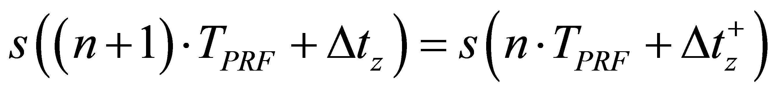
If the target from depth z1 and corresponding signal delay Dtz+ has moved from its previous observation to depth z2 and corresponding time delay Dtz, it can be written (1):
 (1)
(1)
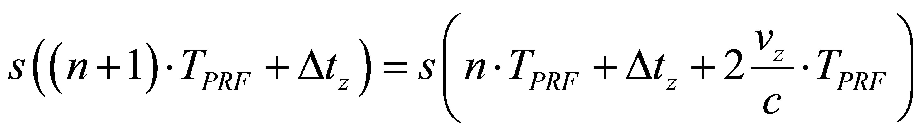
which express the fact that the signal has been slightly shifted between observation n and n + 1, and the acoustic signature observed at depth z1 will be observed at a different depth z2 at the next pulse repetition, assuming the amplitudes are preserved. If the target at depth z was moving at velocity component vz along the Oz axis, the relation between the previous and the next positions delay is
 (2)
(2)
where dz is the displacement of the local target between the two successive shots. Then Equation (1) turns into Equation (3)
 (3)
(3)
which is the simple expression of the time delay between the corresponding acoustic signatures of the target between two pulses transmissions. Equation (3) can be then transferred to the frequency domain using the Fourier transform.
The discrete Fourier transform [16] of a signal consists of a complex vector containing amplitude and phase of each of the frequency components. A shifted signal will have the same Fourier amplitude as the original but the phase value will differ by the corresponding phase shift introduced, which is trivial in signal processing.
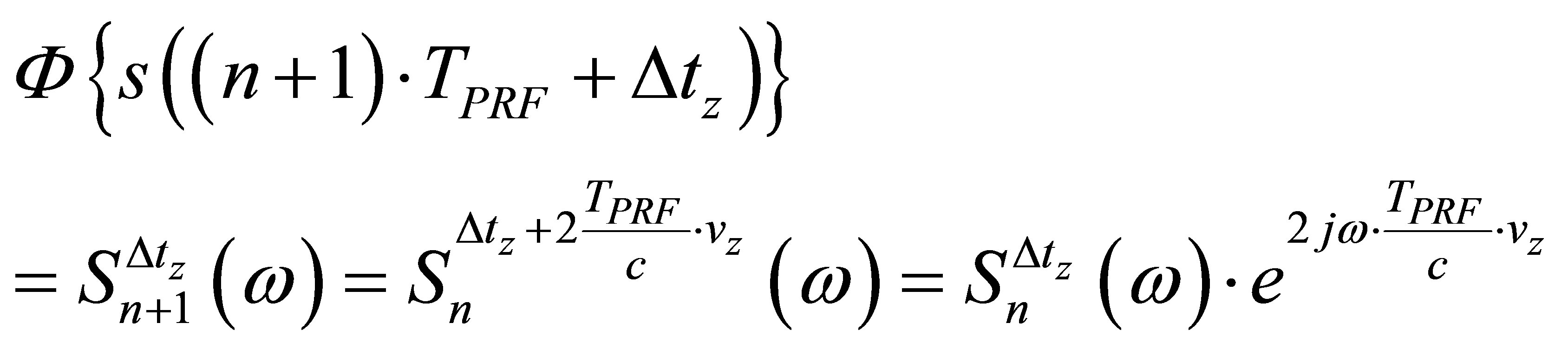
The transform from the time domain to the frequency domain is performed in Equation (4) where F {} denotes the Fourier transform and  is the Fourier transform of signal s at repeat n+1 and depth Dtz
 (4)
(4)
where the time delay appears as a phase shift. Then the delay into the Fourier domain can be simply expressed through spectral division as provided by Equation (5)
 (5)
(5)
and the velocity of the target is then given by Equation (6)
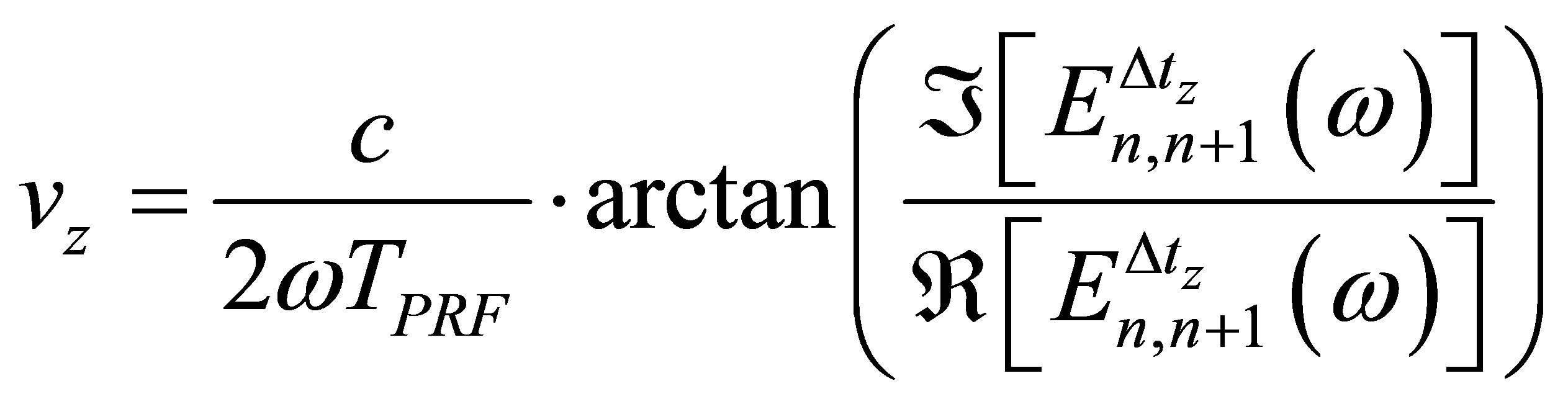 (6)
(6)
where Á {} denotes the imaginary part and  {} the real part.
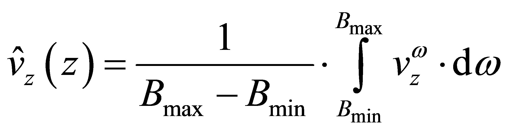
Equations (4) to (6) imply that the local velocity can be deduced from each frequency in the data segments. Thus each frequency is a potential estimator  of the real local velocity component vz, its final estimate
  being the mean value of
  for each available frequency w.
  is expressed in Equation (7), where the measured signal is assumed to be band-limited between Bmin and Bmax, and the estimates at each frequency are integrated and averaged over the bandwidth:
 (7)
(7)
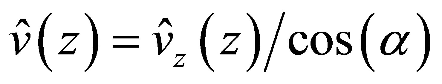
which gives Equation (8) after reordering the terms and introducing the incidence angle a between the ultrasound beam and the flow:
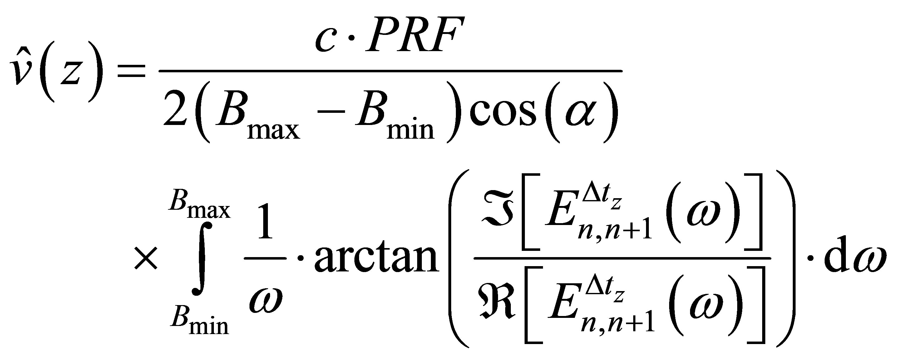 (8)
(8)
 is the local velocity estimate which must be evaluated at each depth z. The bandwidth estimation is important as the phase information doesn’t have any meaning outside the bandwidth (i.e. in the noise signal), which is the standard issue in spectral division. However the technique is still valid for more complex “bandwidths”, which could well be defined over several sections of the spectrum. Equation (8) is the proposed Phase Fourier Doppler (PFD) estimator, which gives its strength to the proposed approach through combining the information at several frequencies to produce an improved estimate of the local velocity. Even with a small bandwidth, n available frequencies as much improve the accuracy of estimation and the need for Doppler lines repeats.
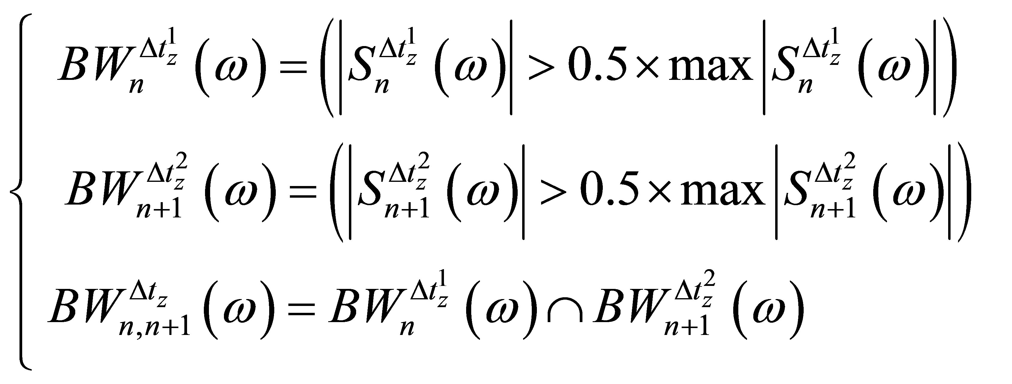
Assuming that the bandwidth definition is at half the amplitude (−6 dB) of the maximum spectrum peak, the integration domain is computed in the following study using (9)
 (1)
(1)
where  is the domain of definition of the integral of the estimator, which can be seen for evaluation purposes as logical map equal to 1 inside the bandwidth of
 , and zero otherwise, and
  the intersection domain of
  and
and .
.
The Fourier transform can unfortunately not be computed at each depth over a single sample, and an implementation of the proposed method must be performed, alike the other Doppler techniques, on successive segments of data, whose length depends on the desired Doppler resolution and the characteristics of the acquisition. The processing of successive segments with more or less overlapping [3,7,10] allows extracting a velocity profile. This is performed in the following sections after acquiring data using a flow phantom, and comparison is made with basic version of classic velocity estimators.
2.2. Experiments
In order to test the proposed technique, RF ultrasound Doppler data were acquired on a phantom flow system set up in a water tank (Figure 1). The phantom in the imaging region was composed of a latex tube [17] (Penrose drainage tubing, Apexmed International, Netherlands) connected to a centrifugal pump (Eheim Universal Rotary Pump, model 1048, Eheim, Germany) and a rotameter (Cole-Parmer Instruments, UK) to control the flow rate. Cellulose particles (Sigmacell Type 20, SigmaAldrich Co) were added to the water in the circuit at 20 g·L−1 to act as linear scatterers [18] . The data were acquired using an L14-38 Ultrasonix (Ultrasonix, Richmond, Canada) probe on an Ultrasonix RP 500 ultrasound research scanner (Figure 1), and an in-house program allowed the setting of the different acquisition parameters and the recording of the raw radio frequency data. The latex tube was 8 mm in internal diameter, 200 mm thick, and 50 cm in length to allow the flow to develop. Data were recorded at around 40 cm from its inlet at flow rates of 300, 400, 500 and 600 cube centimetre per minute (ccm), corresponding to mean velocities of around 10, 13, 17 and 20 cm·s−1 (and corresponding maximum flow speed of ~20, ~26, ~35 and ~40 cm·s−1).
The Reynolds number at the highest flow rate was around Re = 1600 (See for calculation of the Reynolds number with: Mean velocity max: 20 cm·s−1; Characteristic diameter 0.8 cm; Fluid density 1 kg·L−1; Fluid viscosity ~1 cP). With Re < 2000, it is assumed that at the measurement site the flow was laminar and fully developed, with a parabolic velocity profile (while instabilities may start to appear in the flow at the higher flow rates,
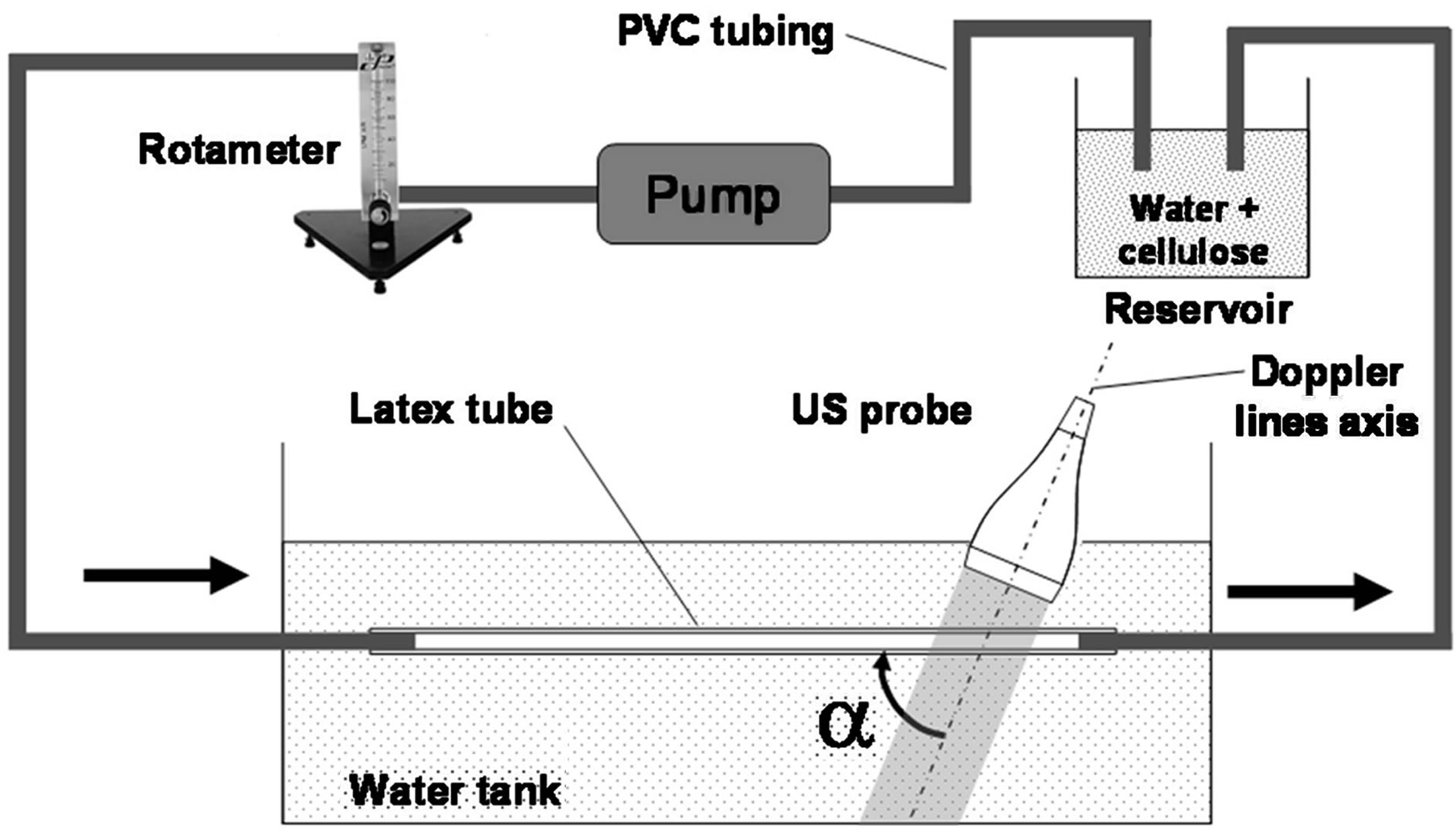
Figure 1. Experimental setup for the acquisition of ultrasound Doppler signals on a latex phantom and a controlled flow of water and cellulose particles. α is the angle between the primary flow and the ultrasound beams.
as the flow gets increasingly disturbed with Re getting higher). Lower and higher flow rates were not achievable, as it was observed that cellulose was starting to decant at lower flow rates, disturbing the flow, and as higher flow rates led to a disturbed/turbulent flow and the corresponding flattened flow profile, useless for the study. This last point was likely due to the thinness of the pipe (200 µm), which is excellent for ultrasound measurements, but also very sensitive, over a great tube length, to flow disturbances and shear stress.
The ultrasound sequence was defined for a 4 cm acquisition depth for a focus at 2.5 cm, and the transmission was performed at f0 = 5 MHz. The L14-5/38 probe is said by Ultrasonix to have a centre frequency of 14 MHz with 5 MHz bandwidth, but it has been observed to transmit efficiently at 5 MHz. The excitation pulse shape on the Ultrasonix is a square wave controlled through a succession of “+”, “−” and “0”, a “plus” programming a positive rectangular excitation and a ‘minus’ a negative one. The amplitude of the excitation waves was 47 Volts (scanner’s specifications). The data were acquired using a single “+” of 100 ns for the transmission (pulse P1). For each frame, 128 ultrasound lines were acquired for B-mode observation, followed by 256 repetitions of the central line for Doppler processing. The pulse repetition frequency (PRF) was 13.56 kHz. The same acquisitions were performed using a longer excitation (pulse P2) “+−+−“, of total length of 400 ns, to enable comparing the results with a more standard-longer-frequency/phase domain Doppler pulse. Data were sampled at fs = 40 MHz.
In order to allow testing the ability of the proposed method to work also in different frequency bands, after data acquisitions on the cellulose flow, ultrasound contrast agent (UCA) (Sonovue™, Bracco Research Inc., Switzerland) [19] was injected in the flow circuit and the measurements repeated. For the contrast, imaging the pulse P2 was used to increase the energy transmitted through the bubble cloud and the contrast response.
2.3. Processing
The angle a between the flow and the ultrasound beams was estimated on the B-mode image (see Figure 3-left). For each flow rate, the data were parsed in segments into successive 93.75% overlapping segments of 64 samples. The choice of this latter parameter is discussed further in the discussion. Fast Fourier transforms were systematically computed on twice the number of points in the data segments (i.e. 128 points for 64 samples segments).
The data were processed using the method presented earlier and results compared with one derived from the mean angular frequency of the spectral Doppler (SD) spectrum [5,6] and the autocorrelation (AC) [5,7,20] methods which also are fundamental frequency/phase domain techniques. The estimates are calculated for each algorithm for the same data segments and overlapping ratio, and the estimates compared with the fitted ideal parabolic flow profile. As elaborated versions of SD and AC methods exist, each method was computed in its basic form to account only on its fundamental ability to extract flow information from the data provided; equally, PFD is computed using the equations provided, without attempting to optimize any of the estimation steps. Furthermore, no wall filter was included in the different estimators to compare their natural ability to handle wall and near wall imaging. For the proposed Phase Fourier Doppler algorithm, the Doppler lines were taken by successive couples from a total Doppler lines number Nl, and the mean flow velocity profile and the standard deviation estimated from the successive estimations.
The AC and SD values were estimated in each data segment after quadrature demodulation at the centre transmit frequency (5 MHz) using a Matlab Blackman lowpass filtering, resulting in the generation of the complex Doppler signal. The AC values were derived from the phase of the cross-correlation of the local Doppler signal at lag 1 ([5] -Equation (3)). For the SD estimator, the Doppler spectrum was transformed in power spectrum before computing the mean angular frequency using Equation 3.10 in the Atkinson and Woodcock [6] and estimating the mean local flow velocity (Equation 3.11). For the calculation of the estimates, each technique was provided exactly the same amount of data in terms of number of RF Doppler lines repeats and segments.
The estimations were performed for all flows using different numbers of Doppler lines Nl, from 2 repeats, the minimum, up to 256, the total Doppler lines repeats acquired. The distance to the theoretical parabolic flow profile was computed for all techniques through the mean of the root of the mean square error (Mean RMS Error or M-RMS-E) between the mean flow profile and the theoretical profile for all flow rates. In other words, the final error parameter measured is the mean error for all flow rates, so that each technique accuracy is not assessed on a single profile estimation, but on its global performance over several flow profiles of different rates and function of the number of Doppler lines repeats provided to each algorithm.
In the case of contrast agent imaging, the data were band bass filtered around the harmonic of the 5 MHz transmitted frequency, that is between 8 MHz and 12 MHz, in order to process the nonlinear components of the acoustical response.
3. Results
Examples of ultrasound B-mode image and of a set of Doppler lines are presented in Figure 3. The angle between the flow and the ultrasound beams was estimated (Figure 3-left) to be a = 71˚. Examples of PFD processing steps of two successive data segments are provided in Figure 2. The amplitudes of the spectra of the data segments are displayed in Figure 2(a), where the band limited aspect of the acquisition can be observed. Figure 2(b) shows the corresponding phase information for all frequencies between 0 and fs/2. Figure 2(c) displays the integration domain selected from Equation (9), and Figure 2(d) the raw vector of velocities estimated from the phase information at all frequencies, before integration and averaging over the bandwidth domain. The estimates are uncorrelated outside the bandwidth of the system, inside which the velocities are marking a kind of plateau indicating the strong correlation between the speeds estimated in the bandwidth domain.
3.1. Cellulose Flow Results
The M-RMS-E estimation results are displayed in Figure 4. Globally its amplitude decreases when the number of Doppler lines processed is increased, the average profile tending towards the ideal parabolic profile. The AC method has a smaller M-RMS-E than the SD method when the number of Doppler repeats performed is small, but when the number of lines is increased, both approaches obtain sensibly the same results. The PFD also benefits from increasing the number of Doppler line repeats fed to the algorithm, but its M-RMS-E is smaller than the one from SD and AC. When more than around 10 Doppler repeats are processed, this error does not decrease much further.
It can be noticed that for an increasing number of Doppler lines processed, the SD method seems to require a minimum of Doppler lines repeats between 25 and 60 to provide stabilized estimates, and increasing the number of lines does not further improve the estimation significantly. The AC method performs slightly better for a small number of Doppler lines and only needs about ten lines to reach the SD method stabilized regions, however providing up to 50 lines still improves the estimation.
The instability and noisiness of the SD and AC results for small number of data lines and the impossibility of plotting clear error bars graphs in flow profile estimations led to the sole computation of their mean values over the total number of Doppler lines repeats Nl computed. This mean profile is the one used for error assessment in and accuracy comparison in Figure 4, and it is compared to the parabolic profile.
The PFD errors present the same trends, and processing more data allows to improve the estimations, however the initial 2 Doppler lines are sufficient (Figure 4) to obtain an error smaller than the ones of the two other
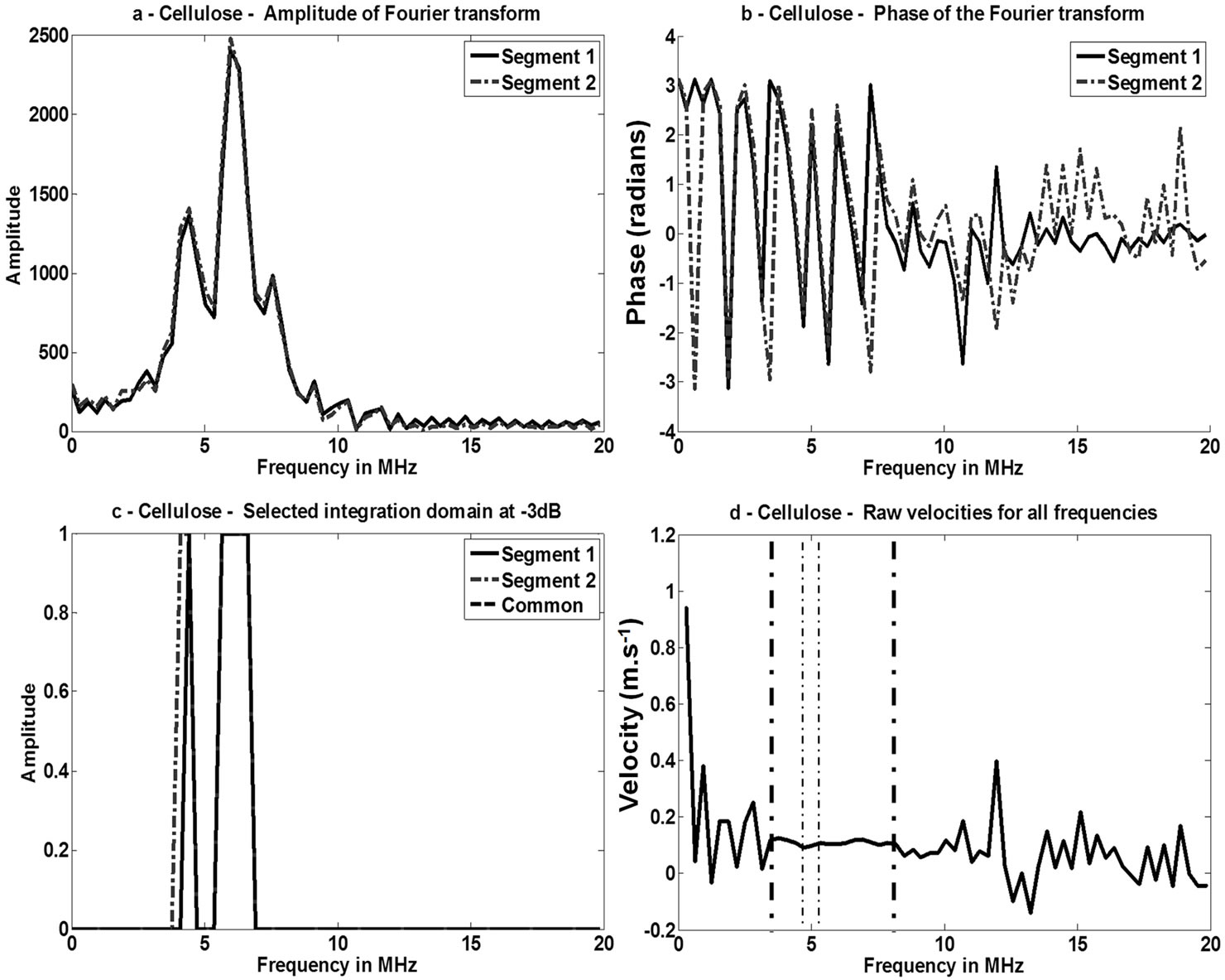
Figure 2. Examples of processing steps on two successive data segments in the middle of the flow while imaging linear-cellulose-particles: a) amplitude of the Fourier transform using the FFT algorithm; b) phase vector information of the Fourier transform; c) −6 dB amplitude-derived piecewise integration domain; d) raw vector of velocities estimated from the phase information before integration and averaging, with delineation of the bandwidth.
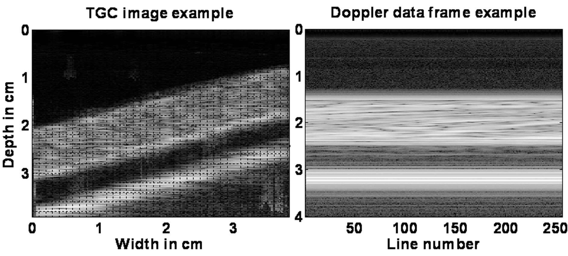
Figure 3. Example of Time Gain Compensated (TGC) Bmode image of the latex tube perfused with water and cellulose (left), and example of Doppler frame (right): the same line is repeated at maximum PRF; the second wide white band which can be observed is an artifact.
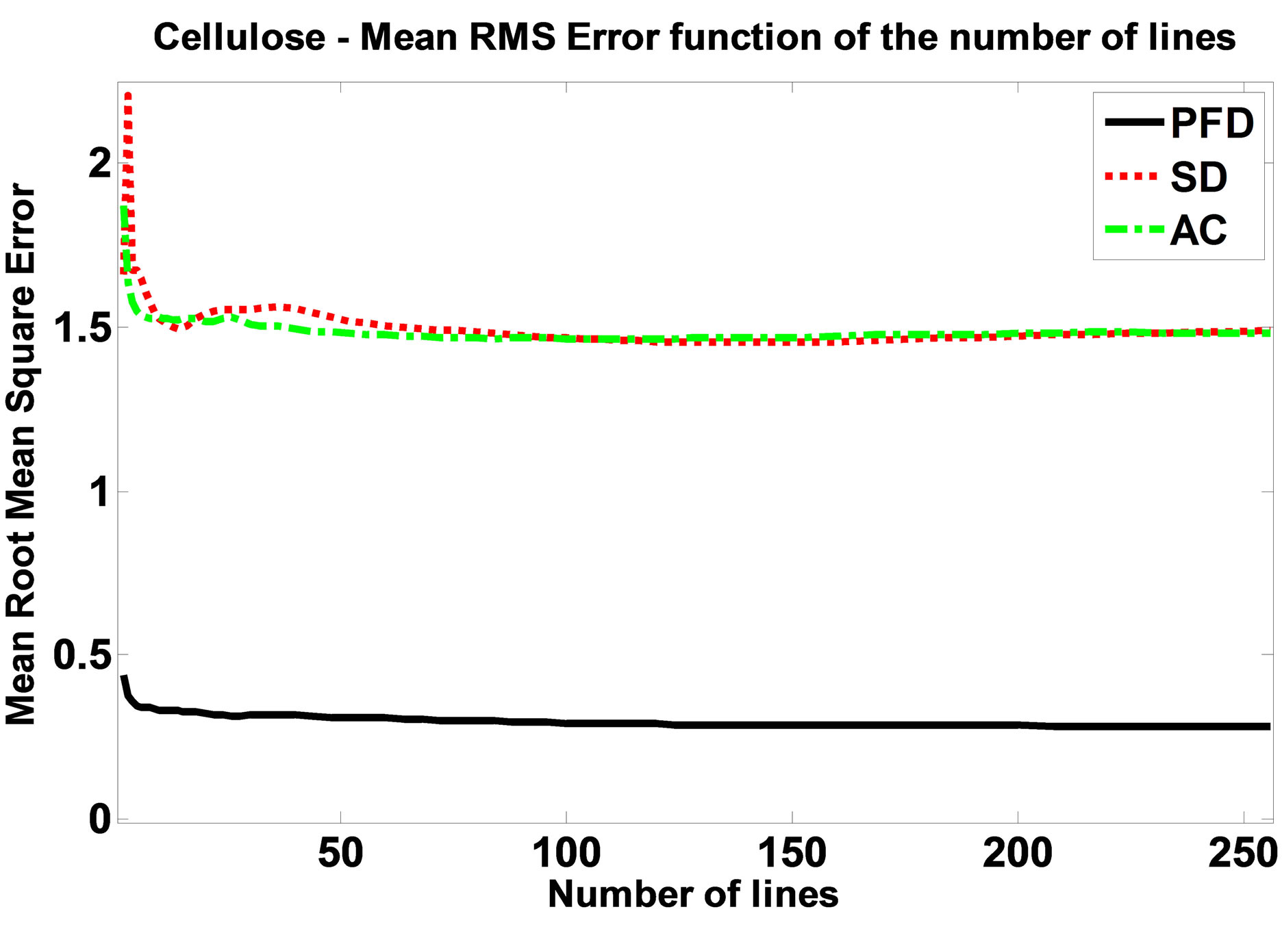
Figure 4. Mean RMS error between the theoretical parabolic profile and the mean profile estimated for each technique (PFD, Spectral Doppler and Autocorrelation), tested at different number Nl of Doppler lines processed for the P1 pulse.
techniques. A slight improvement of the PFD estimates can be observed when up to 10 Doppler lines are processed, and then increasing the number of lines does not seem to improve the estimations significantly.
Flow profiles for each flow rate are displayed in the best (in term of available information) Nl = 256 (Figure 5) and worse Nl = 2 (Figure 6) case scenario; error bars of the PFD estimates were displayed every 5 points for legibility. In Figure 5, the PFD, AC and SD profile are very close to the theoretical parabolic profile, despite the estimation irregularities observed for SD.
The standard deviations of the PFD estimates are not negligible and remain appreciatively the same across the flow profile. However it can be noticed that the AC and SD estimates oscillate inside or very close to the standard deviation domain of the PFD. A small irregularity - possibly a flattening-in the profiles can be observed for the estimates for the 600 ccm flow rate, at the top of the parabola.
In Figure 6, the trend is changed when only Nl = 2 Doppler lines are processed, and the SD and the AC techniques provide nearly the same estimates and diverge at the same locations, while the PFD remains close to the parabolic profile. This is consistent with the mean RMS errors observed in Figure 4, the PFD making a greater error than with Nl = 256, but still performing better than the SD and AC methods which present great estimation errors.
The MRMS results for cellulose flow using pulse P2 are displayed in Figure 7. Error estimation results provided by the use of a longer pulse P2 (“+−+−”) exhibited the same shape as with pulse P1.
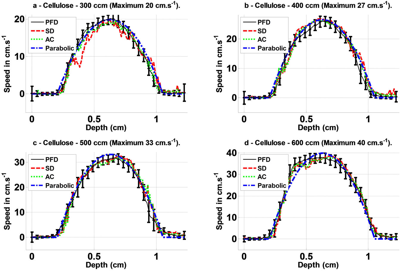
Figure 5. Plots of the estimated flow profiles across the latex tube section (with angle α) and theoretical parabolic profile for each flow rate (a: 300 ccm; b: 400 ccm; c: 500 ccm; d: 600 ccm) imaged using the whole (Nl = 256) Doppler data set.
3.2. Contrast Flow Results
Estimation results for the contrast flow are provided in Figures 8 and 9. Computation results of Mean RMS error to the theoretical parabolic profile as a function of the number of Doppler lines processed (Figure 9) shows that the PFD makes a smaller error than the SD and AC methods, but the benefit is lower than the one obtained at the fundamental in the cellulose results.
The SD and AC error profiles get very close when the number of Doppler lines processed is increased, but the AC errors tend decrease more rapidly. On another hand, when the number of Doppler lines processed is drastically reduced, the PFD error is close to the one obtained from SD and AC for a large number of Doppler lines.
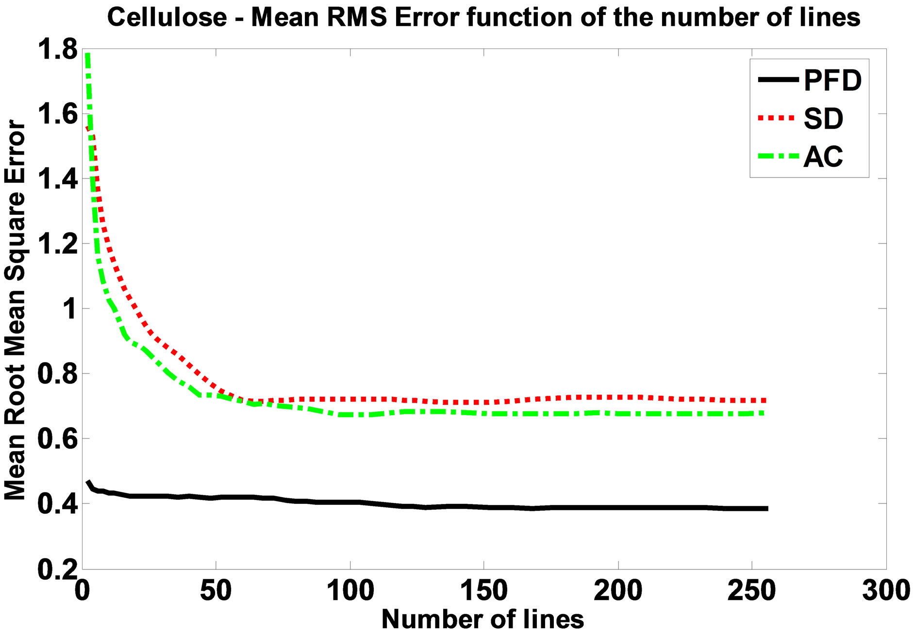
Figure 6. Mean RMS error to the parabolic profiles using the “+−+−” narrower bandwidth pulse.
This is further illustrated in Figure 8 where the estimated profiles and the theoretical parabolic one have been plotted for the 300 ccm and 600 ccm flows for both Nl = 2 and Nl = 256 Doppler lines processed. The estimates of the PFD inside the flow for the Nl = 2 lines are a bit noisy but remain globally parabolic and closer to the theoretical profile than the SD and AC estimates. It can be noticed, especially in the Nl = 256 and 600 ccm flow rate case, that the estimated flow velocities are slightly smaller than the theoretical values.
4. Discussion
4.1. Cellulose Flow Results
The smaller errors exhibited by PFD in Figure 4 suggest than the PFD is performing better than the SD and AC. A slight increase of error values can be observed for around 40 Doppler repeats for all techniques, which could be due to flow irregularities, as the latex tube was not held in place and could vibrate and could possibly have an irregular surface state likely to generate flow instabilities. But globally the error is decreasing when increasing the number of lines processed. In Figure 5, the standard deviations of the PFD estimates are not negligible and remain appreciatively the same across the flow profile. A small irregularity in the profiles can be observed for the estimates for the 600 ccm flow rate, at the top of the parabola. This can be due to the approximate setting of the flow given the imprecision of the manually-set rotameter, but it is believed to be due to flow irregularities or to the beginning of the turbulence/instability in the flow, the
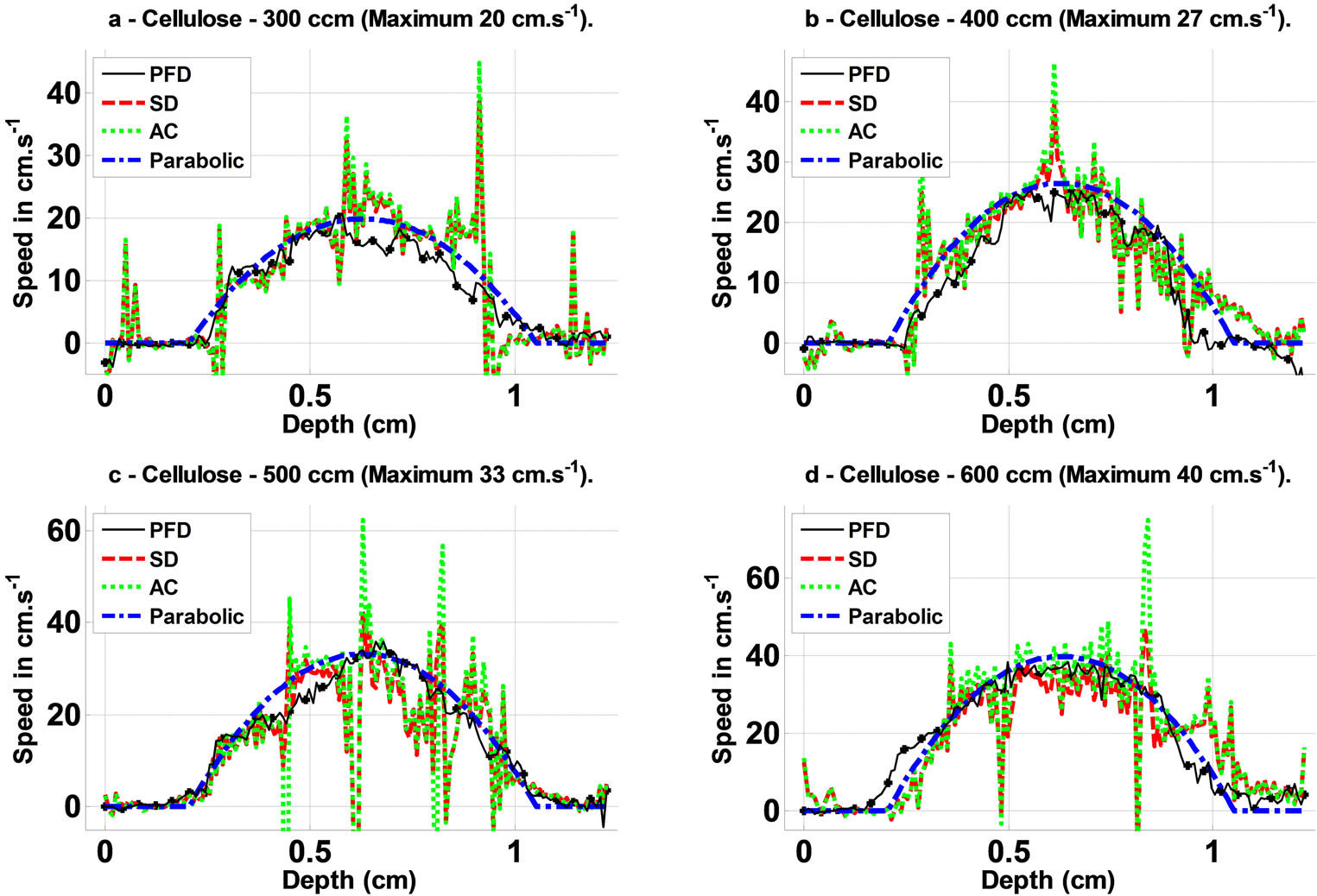
Figure 7. Plots of the estimated flow profiles across the latex tube section (with angle α) and theoretical parabolic profile for each flow rate (a, 300 ccm; b, 400 ccm; c, 500 ccm; d, 600 ccm) imaged using only Nl = 2 Doppler lines.
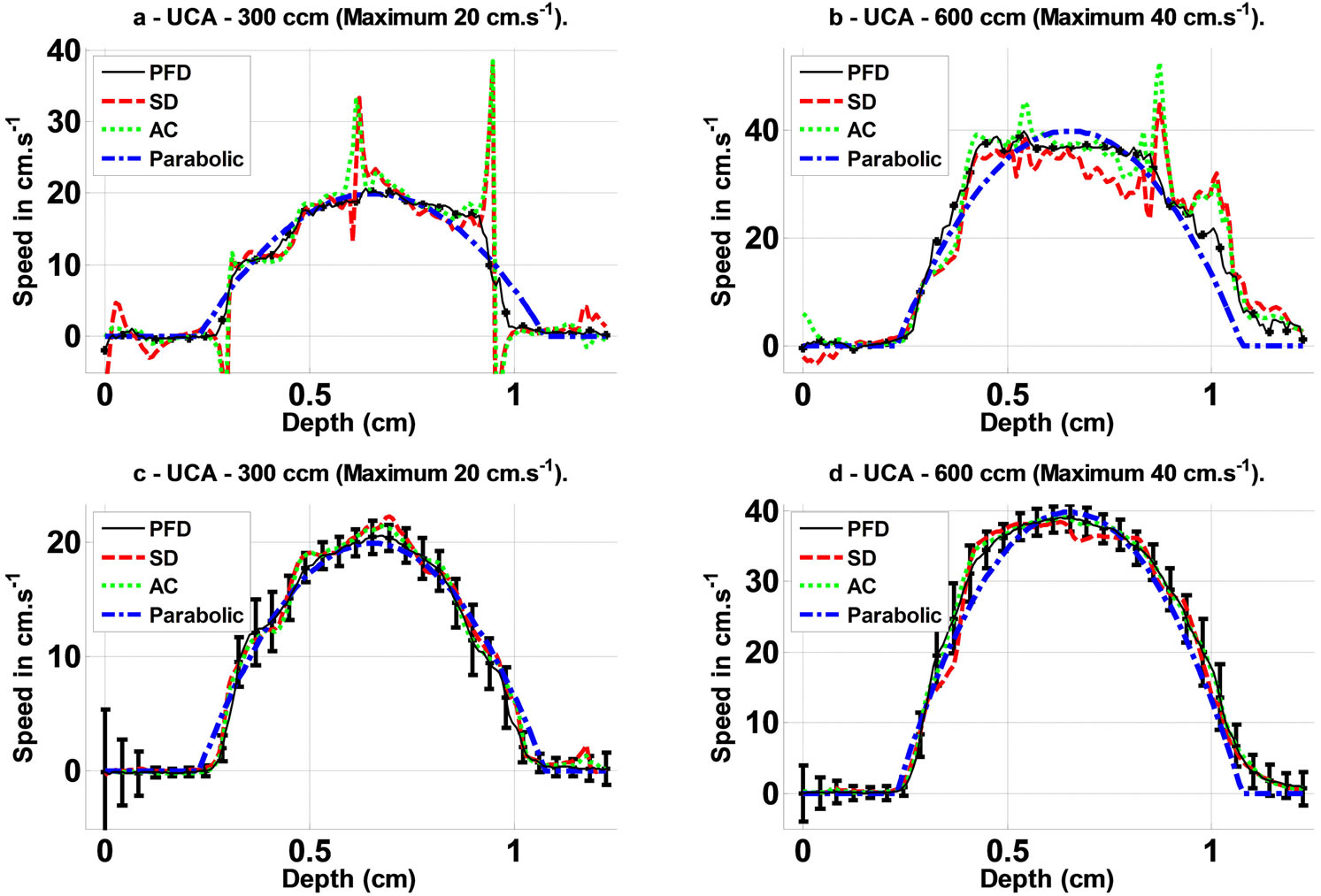
Figure 8. Post UCA-injection plots of the estimated flow profiles across the latex tube section (with angle α) and theoretical parabolic profile for flow rates 300 ccm ((a) and (c)) and 600 ccm ((b) and (d)) imaged using Nl = 2 Doppler lines ((a) and (b)) and Nl = 256 Doppler lines ((c) and (d)).
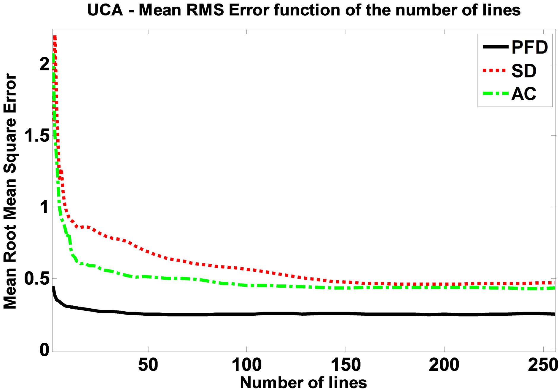
Figure 9. Post UCA-injection Mean RMS error to the parabolic profiles for UCA data filtered in the 8 - 12 MHz band using the P2 (“+−+−”) narrow band pulse.
trend continuing at the greater flow rates, and coherently between all the estimation techniques, with the appearance of a flattened flow profile (not shown), which made the comparison with a theoretical profile impossible.
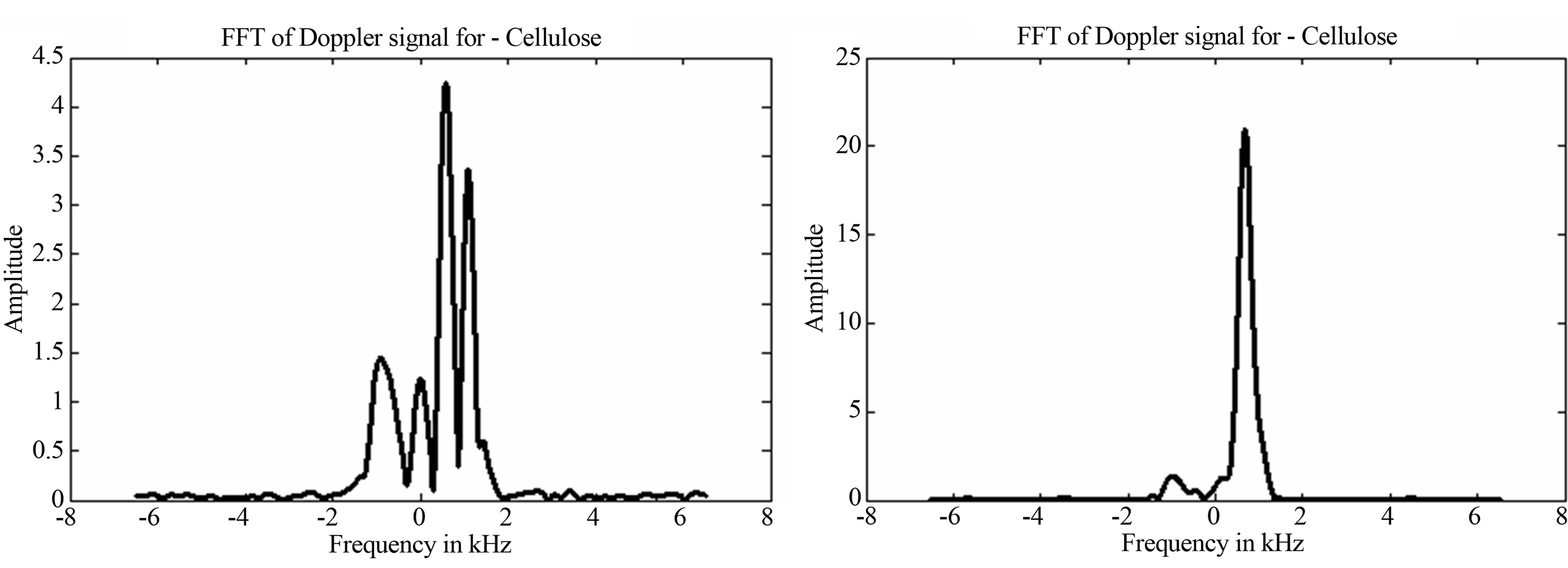
In Figure 6, when only Nl = 2 Doppler lines are processed, the SD and the AC techniques provide nearly the same estimates and fail at the same locations, while the PFD remains closer to the parabolic profile. Once again this result is consistent with the mean RMS errors observed in Figure 4, the PFD making a greater error than with Nl = 256, but still performing better than the SD and AC methods which present larger estimation errors. The increased stability of PFD over the other techniques can be explained by looking into the processing signals in detail and reinterpreting the PFD equations. The raw velocity estimates (for all the frequencies in the spectrum) from the PFD processing were extracted for the segment corresponding to the maximum SD error observed for the 400 ccm flow rate experiment (maximum SD peak in Figure 7(b)). Figure 10(a) shows that in this particular segment, the 5 MHz signal is missing, and such behaviour have been observed to occur in an unpredictable manner. It is due, as shown by Eriksson, et al. [14] , Loupas, et al. [21] , Alam and Parker [4] and Ferrara and al. [22] , to specific frequency cancellation during the local interaction of the propagating pulse with the local scatterers profiles. When demodulating at the expected–and missing–frequency, as illustrated in Figure 11(a), it translates, in the Doppler spectrum domain, into the generation of an unsuited spectrum and, in this case, in the presence of a strong near-zero centered peak, which leads the algorithm to misestimate the local flow velocity.
Demodulation of the same data on the same location at a different frequency, 4 MHz, which was present in the local spectrum, led to a restored accurate estimation of the local flow velocity (Figure 11(b)). However demodulating the whole data set at 4 MHz does not improve the overall estimates, and errors simply occurred at different locations. This underlines the fact that the local frequency content determines the ability of single frequency processing algorithms to perform a correct Doppler estimation. As SD and AC methods are programmed to work (demodulate) at a single frequency, they fail to
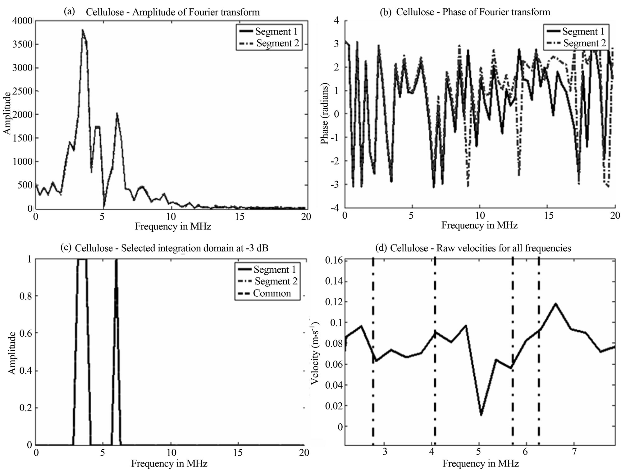
Figure 10. Examples of processing steps on two data segments inside the flow in the case where the 5 MHz frequency component is missing: a) amplitude of the Fourier transform; b) phase vector information; c) −6 dB amplitude-derived piecewise integration domain; d) raw vector of velocities. The PFD approach performs on the stronger frequency components of the data, avoiding (c) the 5 MHz issue and providing more stable estimates.
 (a) (b)
Figure 11. Amplitude of the Doppler signal for a data location where the 5 MHz carrier was found missing or small demodulated at 5 MHz (a) and Doppler spectrum at the same location for a 4 MHz demodulation (b); demodulation at a frequency locally present leads to correct velocity estimation.
estimate the flow rate properly at some locations if the frequency is not adapted to the local changes, and generate localized but significant errors.
Alam and Parker [4] showed that the butterfly search can overcome these irregularities, but it implementation requires the observation of several Doppler lines to track the acoustic signature of a moving scatterer. On the other hand, Eriksson [14] proposed to solve the problem by transmitting at different frequencies and averaging the estimates, which is a good first approach, but further reduces the frame rate and the Doppler images resolution. Furthermore doing so requires the demodulation of each transmission at its own frequency, while Figure 11, and the PFD approach in general, show that a single transmission would have been sufficient while demodulating at several ones. The PFD method does this naturally at a lower computational cost by first analyzing the spectral content and averaging the velocity information over the values which have a sufficient spectral energy, avoiding the processing of noise and averaging the estimates over several other frequencies. It is in this aspect that PFD can provide significantly improved estimates compared to the other phase domain techniques: it uses more of the available information of the signal. It is less sensitive to local errors and if one of the frequencies present in the spectrum is having an ill-defined phase information, it will be, in the worst case, averaged with the other ones, maintaining a greater stability of the estimates.
The drawback of this aspect is that the local amount of information used by the PFD is changing all the time, at least with the current implementation, so that each estimate is the result of an averaging over a different number of values, leading to inequalities in accuracy inside a given velocity profile. This could be avoided by limiting the number of values considered before averaging, but in the end would simply lead to worse estimates. The SD and AC method could also be corrected to avoid situations of divergence; for example the demodulation could be performed at different frequencies, in order to provide a mean estimate instead of a single one. However this would still lead to the processing of locally ill-defined frequencies, which would contribute to local divergence. Further stability could be achieved by performing a local estimation of the frequency content, but this would be equivalent to the minimum computation of a local FFT processing, which would be close to a PFD process. However the use of a longer pulse P2 (“+−+−”) did not significantly change the results obtained previously with the shorter pulse which can be transmitted by the scanner (Figure 7). Finally the estimation results have been provided without any spatial filtering despite the fact that this is usually performed on ultrasound scanners to display a smoothed profile, which explains the sometimes chaotic aspect of the estimates displayed in the present study. However the high frequency content of the faster flow requires being able to perform Doppler imaging without smoothing out this content too much, or the resulting flow which is imaged is an average which ignores the local variation in space and time.
4.2. Contrast Flow Results
In the case of contrast imaging, the errors differences, as plotted in Figure 9, have the same global trends as the ones obtained from cellulose flow, and the PFD performs globally better than the other techniques, but difference of M-RMS-E is smaller. This is due to the bandpass filtering of the signal around the harmonic response in the spectrum: fewer frequencies are available for averaging to the PFD algorithms. This illustrates the limits of the bandpass filtering combination of the PFD, which gains its efficiency from the availability of many frequencies over which the local estimate is averaged. But its capacity to perform better with fewer Doppler repeats still makes the approach of interest for fast Doppler estimations in the case of narrow bandwidth computations.
The estimates in the wall in all estimations present (Figure 8) greater errors compared to the estimates provided on the cellulose flow and the standard deviations are also greater; this is likely due to a nearly complete absence of harmonic response in the wall and corresponding low signal to noise ratio in these locations. This is also a consequence of the limitation of the current version of the proposed technique through the absence of wall filtering: when the signal to noise ratio is too small, the bandwidth of the signal is not well defined, and the current domain of averaging of the estimates tends to include noise components.
However, the results demonstrate that the proposed technique can be used to compute the velocity profile in arbitrary frequency bands of the received signal, allowing it to combine with contrast imaging approaches. Further research in this matter should attempt to apply the PFD algorithm with non-linear imaging techniques such as Phase Inversion, Amplitude modulation or combined techniques [20] , and for example, to process the residual signals, and also to develop dedicated wall filtering techniques. But it should be noticed that regarding the standard application of the technique which include the processing of the linear part of the backscattered signal, the PFD approach naturally performs wall filtering (no continuous component as in SD) and can also be used for tissue Doppler measurements (but it does not implements intrinsically noise rejection).
4.3. General Discussion
An additional interesting aspect of the PFD is the possibility to obtain better Doppler resolution through the use of short pulses. Indeed, “standard” long pulses tend to spread and mix the responses of neighbouring scatterers, rendering each estimation window more likely to sense the velocities of the adjacent ones. The use of short pulses limits this spreading effect, making the flow estimates more local, which adds to the improved accuracy of the proposed technique.
But it should be noted that the present expression of the bandwidth selection (Equation (9) for the averaging of the velocity estimates does not take into account the fact that too high transmit frequency cannot be used if the local displacement is greater than half the corresponding wavelength. This is partly solved by the use of very high PRF, and it also works well with band limited pulses as the greater frequencies of the Fourier spectrum are supposed to be null. But in the hypothetical case of a perfect ultrasound impulse, even with an amplitude well defined, for a given PRF, the local velocity fixes the upper bound of the usable averaging domain, which is the ultimate limit of the PFD and of Doppler techniques in general.
Furthermore, the proposed implementation is appropriate for band limited pulses, which is suitable for ultrasound imaging, but cannot be applied straightforwardly to any kind of image, and would need to be adapted in different conditions of signal elaboration.
A shift appears in the calculation of the errors for all techniques, but the error of the PFD approach is lower. This is likely due to the fact that the PFD process averages the estimates through different frequencies, and suppresses the ill-defined ones, allowing to reduce the instabilities in the estimates, through this achieve a much lower mean error compared to the standard methods.
It should be noted that a single segment length, or gate size, (i.e. 64 samples segments) was tested in this study, which resulted from a compromise between spatial resolution and samples requirements for the calculation of the Fourier transform. The corresponding gate size is 1.6 µs, which can be compared with the 1 µs to 3 µs gates lengths range found in the Cobbold [13] manual chapter 9. While the number of samples available depends also on the sampling frequency used for the RF acquisition, a complete study of this parameter remains to be performed.
Finally, the proposed technique has been compared with basic implementations of the main estimator, SD and AC, while refined versions may prove more successful. However this permitted to account for their natural capacity to extract flow information from the RF data. Future implementations of the PFD may improve the proposed one, like SD and AC benefited from advanced or dedicated implementations. Future work should also consider comparison of the techniques in combination with a wall filtering, to account for their different abilities to include such step in their processing.
5. Conclusion
Standard pulsed Doppler techniques such as spectral Doppler or autocorrelation are limited by their single frequency approach and B-mode/Doppler spatial resolution due to the corresponding long pulses used for transmission. A Doppler method is presented that estimates the shifts between successive Doppler line segments using the phase information provided by the Fourier transform. In order to test and assess the performance of the proposed technique, signals were acquired with an Ultrasonix RP500 research scanner in a straight latex pipe perfused with water and cellulose scatterers. To compare the abilities of the technique with the existing phase domain Doppler approaches, the estimation results are computed along with the velocity estimates provided by standard-phase domain-spectral Doppler and autocorrelation methods, for different number of Doppler lines processed. The Mean RMS Error to the theoretical parabolic profile is computed for different flow rates properly developed using their mean estimates of each technique. Results show that the proposed method performs better than both spectral Doppler and autocorrelation techniques, especially when few Doppler lines are processed. This improved accuracy is due to extraction of more information from the backscattered signals, as the estimates are performed at multiple frequencies. If the use of a single frequency for estimation makes sense when continuous wave Doppler is performed, the standard pulsed Doppler approaches have wider band pulses while they rely on a single frequency only. This renders the velocity estimation dependent of the stability of that frequency in the backscattered signal, and requires increasing the number of Doppler lines repeats, which ultimately lowers the frame rate. It was shown that a phase domain Fourier approach can overcome that limitation by extracting multiple frequency information, through a combination of spectral division and averaging of the frequency dependent velocity estimates over the bandwidth. A possible drawback of the technique proposed here is that it does not produce a local Doppler spectrum detailing the range of velocities imaged in the Doppler resolution cell, and that it requires the estimation of the local bandwidth of the system. But regarding this latter point, results show that problems only occur when no signal is present, which is a typical weakness of Doppler techniques in general. As stated previously, one of the further strengths of the proposed technique over the other phase-domain ones is that it allows performing Doppler imaging with very wide-band pulses, which makes it able to gain in both B-mode and Doppler resolution, while providing more reliable velocity estimates. Through injection of Sonovue® microbubbles in the system, it was demonstrated that this Doppler approach is compatible with nonlinear imaging techniques. Further research will attempt to combine it with the recently developed non-linear Doppler techniques, to handle the low signal-to-noise ratio situations, and of course to perform in vivo data processing. Despite the remaining limitations, Phase Fourier Doppler is a rare case of efficiency of spectral division and a significant step toward high resolution, high speed and high accuracy ultrasound Doppler, which demonstrates that ultrasound imaging continues to be a progressing modality full of promises.
6. Acknowledgements
The author thanks Professor Colin G. Caro and Dr. Adrien Desjardins for their support. This work has been originally funded by the Garfield Weston Foundation and the Henry Smith Charity (UK).
REFERENCES
- C. G. Caro, J. M. Fitzgerald and R. C. Schroter, “Atheroma and Arterial Wall Shear—Observation, Correlation and Proposal of A Shear Dependent Mass Transfer Mechanism for Altherogenesis,” Proceedings of the Royal Society, Vol. 177, No. 1046, 1971, pp. 109-133
- T. Yamamoto, Y. Ogasawara, A. Kimura, et al., “Blood Velocity Profiles in the Human Renal Artery by Doppler Ultrasound and Their Relationship to Atherosclerosis. Arteriosclerosis,” Thrombosis & Vascular Biology, Vol. 16, No. 1, 1996, pp. 172-177. doi:10.1161/01.ATV.16.1.172
- K. Ferrara and G. DeAngelis, “Color Flow Mapping,” Ultrasound in Medicine and Biology, Vol. 23, No. 3, 1997, pp. 321-345. doi:10.1016/S0301-5629(96)00216-5
- S. K. Alam and K. J. Parker, “Implementation Issues in Ultrasonic Flow Imaging,” Ultrasound in Medicine & Biology, Vol. 29, No. 4, 2003, pp. 517-528. doi:10.1016/S0301-5629(02)00704-4
- J. A. Jensen, “Algorithms for estimating velocities using ultrasound,” Ultrasonics, Vol. 38, No. 1-8, 2000, pp. 358-362. doi:10.1016/S0041-624X(99)00127-4
- P. Atkinson and J. P. Woodcock, “Doppler Ultrasound and Its Use in Clinical Measurement,” Academic Press Inc., London, 1982.
- C. Kasai, K. Namekawa, A. Koyano and R. Omoto, “Real-Time Two-Dimensional Blood Flow Imaging Using an Autocorrelation Technique,” IEEE Transactions on Sonics and Ultrasonics, Vol. 32, No.3, 1985, pp. 458- 464.
- L. N. Bohs, B. J. Geiman, M. E. Anderson, S. C. Gebhart and G. E. Trahey, “Speckle Tracking for Multidimensional Flow Estimation”, Ultrasonics, Vol. 38, No. 1-8, 2000, pp. 369-375. doi:10.1016/S0041-624X(99)00182-1
- L. S. Wilson, “Description of broad-band pulsed Doppler ultrasound processing using the two-dimensional Fourier transform,” Ultrasonic Imaging, Vol. 13, No. 4, 1991, pp. 301-315.
- J. A. Jensen, “Implementation of Ultrasound Time Domain Cross-Correlation Blood Velocity Estimators,” IEEE Transactions on Biomedical Engineering, Vol. 40, No. 5, 1993, pp. 468-474.
- P. M. Embree and W. D. O’Brien, “The Accurate Ultrasonic Measurement of the Volume Flow of Blood by Time Domain Correlation,” Proceedings Ultrasonics Symposium, San Francisco, 16-18 October 1985, pp. 963-966.
- P. J. Brands, A. P. G. Hoeks, L. A. F. Ledoux, R. S. Reneman, “A Radio Frequency Domain Complex CrossCorrelation Model to Estimate Blood Flow Velocity and Tissue Motion by Means of Ultrasound,” Ultrasound in Medicine & Biology, Vol. 23, No. 6, 1997, pp. 911-920. doi:10.1016/S0301-5629(97)00021-5
- R. Cobbold, “Foundations of Biomedical ultrasound,” Oxford University Press, Oxford, 2007.
- R. Eriksson, H. W. Persson, S. O. Dymling and K. Lindstrom, “Blood Perfusion Measurement with Multifrequency Doppler Ultrasound,” Ultrasound in Medicine & Biology, Vol. 21, No. 1, 1995, pp. 49-57. doi:10.1016/0301-5629(94)00087-5
- J. M. Mari, O. BouMatar, T. Blu, M. Unser and C. Cachard, “A bulk modulus dependent linear model for acoustical imaging,” Journal of the Acoustical Society of America, Vol. 125, No. 4, 2009, pp. 2413-2419. doi:10.1121/1.3087427
- E. Brigham, “The Fast Fourier Transform and Its Applications,” Prentice Hall, Englewood Cliffs, 1988.
- D. W. Rickey, P. A. Picot, D. A. Christopher and A. Fenster, “A Wall-Less Vessel Phantom for Doppler Ultrasound Studies,” Ultrasound in Medicine & Biology, Vol. 21, No. 9. 1995, p. 176. doi:10.1016/0301-5629(95)00044-5
- A. D. A. Christopher, P. N. Burns, J. Armstrong and F. Stuart Foster, “A High-Frequency Continuous-Wave Doppler Ultrasound System for the Detection of Blood Flow in the Microcirculation,” Ultrasound in Medicine & Biology, Vol. 22, No. 9, 1996, pp.1191-1203. doi:10.1016/S0301-5629(96)00153-6
- J. Tu, J. Guan, Y. Qiu and T. Matula, “Estimating the Shell Parameters of SonoVue® Microbubbles Using Light Scattering,” Journal of the Acoustical Society of America, Vol. 126, No. 6, pp. 2954-2962. doi:10.1121/1.3242346
- C. J. Harvey, J. M. Pilcher, R. J. Eckersley, M. J. Blomley and D. O. Cosgrove, “Advances in Ultrasound,” Clinical Radiology, Vol. 57, No. 3, 2002, pp. 157-177.
- Loupas, et al., “An Axial Velocity Estimator for Ultrasound Blood Flow Imaging,” IEEE TUFFC, Vol. 42, No. 4, 1995, pp. 911-920.
- K. W. Ferrara, V. R. Algazi and J. Liu, “The Effect of Frequency Dependent Scattering and Attenuation on the Estimation of Blood Velocity Using Ultrasound,” IEEE TUFFC, Vol. 39, No. 6, 1992, pp. 754-767. doi:10.1109/58.165561