Open Journal of Acoustics
Vol.2 No.3(2012), Article ID:22604,12 pages DOI:10.4236/oja.2012.23015
Feature Extraction for Audio Classification of Gunshots Using the Hartley Transform
Department of Electronics Engineering, Technological Education Institute (TEI) of Piraeus, Athens, Greece
Email: iparaskevas@theiet.org, mariar@teipir.gr
Received August 9, 2012; revised September 6, 2012; accepted September 14, 2012
Keywords: Hartley Transform; Hartley Phase Spectrum; Frequency Domain Feature Extraction; Classification
ABSTRACT
In audio classification applications, features extracted from the frequency domain representation of signals are typically focused on the magnitude spectral content, while the phase spectral content is ignored. The conventional Fourier Phase Spectrum is a highly discontinuous function; thus, it is not appropriate for feature extraction for classification applications, where function continuity is required. In this work, the sources of phase spectral discontinuities are detected, categorized and compensated, resulting in a phase spectrum with significantly reduced discontinuities. The Hartley Phase Spectrum, introduced as an alternative to the conventional Fourier Phase Spectrum, encapsulates the phase content of the signal more efficiently compared with its Fourier counterpart because, among its other properties, it does not suffer from the phase “wrapping ambiguities” introduced due to the inverse tangent function employed in the Fourier Phase Spectrum computation. In the proposed feature extraction method, statistical features extracted from the Hartley Phase Spectrum are combined with statistical features extracted from the magnitude related spectrum of the signals. The experimental results show that the classification score is higher in case the magnitude and the phase related features are combined, as compared with the case where only magnitude features are used.
1. Introduction
The spectral magnitude information reveals how the energy content of a signal is distributed across the frequency spectrum, i.e., the signal energy concentration across frequencies. The magnitude spectrum ignores the information related to the location of the aforementioned magnitude spectral components in the time domain. The information related to the location of the signal magnitude characteristics in the time domain as well as to the signal dynamics is encapsulated in the phase spectrum [1,2].
Not until relatively recently, researchers in music processsing [3], sound source separation [4], biomedical engineering [5], speech/word recognition [6] and speech processing [7] have emphasized on the usefulness of phase and proposed the use of the phase spectrum. Specifically, the phase spectrum is used for various speech processing applications such as formant extraction, pitch extraction, speech intelligibility, speech enhancement, iterative signal reconstruction and automatic speech recognition [1,2,6]. The conclusions derived from the review in [1] indicate that, for the automatic speech recognition application, the (processed) phase spectrum encapsulates class discriminative information not conveyed by the signal magnitude (e.g. the Mel-Frequency Cepstral Coefficients (MFCCs)). Moreover, in the same work it is stated that, in case feature vectors are extracted from both the magnitude and the phase spectra of speech signals, the recognition performance and class separability should be improved. The experimental results of the present work, for classification of audio signals, agree with both the aforementioned claims.
Hence, the aim of the present work, which is focused on the frequency domain feature extraction for audio classification, is to show that the combination of the magnitude with the phase spectral information provides higher classification scores compared with the case when only magnitude information is used.
The phase spectral function conveys discontinuities that are caused either due to artifacts which are not related to the signal, [8] or due to certain characteristics the signal conveys (Subsection 2.1) [9]. In this work, methods are developed that eliminate the aforementioned discontinuities from the phase spectrum. The experimental results indicate that the discontinuities of the phase spectrum affect the recognition performance; indeed, it is seen that the classification scores increase with the reduction of discontinuity occurrences.
In [10], the phase and magnitude features combination was shown to be advantageous in terms of recognition performance; however, phase computation via the Fourier Transform could not adequately address the phase discontinuities problem. The Hartley Transform employed here leads to a phase spectrum that suffers fewer discontinueties while it encapsulates the phase content of the signal in an improved manner; moreover, it yields robust features in the presence of noise.
Briefly, in this work three alternative frequency domain feature sets are selected and then used in combination for classification; these are extracted from: (a) The Fourier Magnitude spectrogram; (b) the Hartley Magnitude spectrogram; and (c) the Hartley Phase spectrogram.
Their relative merits for classification are tested on a set of acoustic signals from a database containing acoustically similar sounds (“fine” audio classification application). Specifically, in this work the acoustic signals employed are gunshots. This audio dataset is chosen intentionally due to the similarities that the gunshot classes exhibit in terms of their magnitude spectral content (Figures 1(a) and (b)); therefore, features should also be extracted from their phase spectrum. The experimental results in Section 5 show that the combination of the aforementioned feature sets (a), (b) and (c) increases the classification scores significantly, as compared with the independent feature set case. Details on the database used and on the characteristics and similarities of the signals are provided in Section 4.
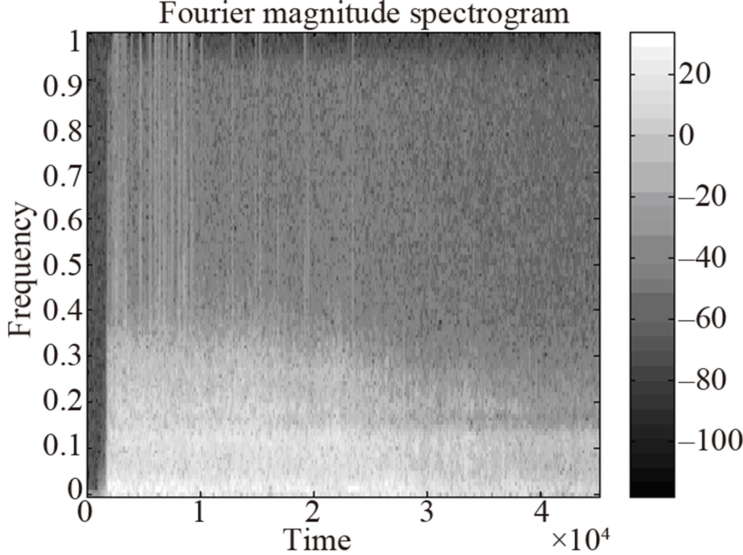 (a)
(a)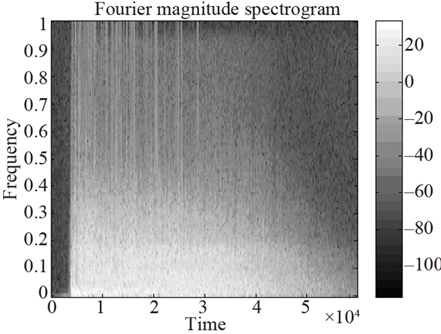 (b)
(b)
Figure 1. (a) Fourier Magnitude spectrogram of a 30 - 30 rifle shot recording; (b) Fourier Magnitude spectrogram of a pistol shot recording.
Furthermore, an important issue that arises is whether parametric features, such as the MFCCs, typically employed in order to compress the magnitude content of speech and audio signals [11], reach a higher classification rate compared with the aforementioned combinatory scheme, given that the MFCCs encapsulate purely magnitude content of the signal whereas, the proposed scheme encapsulates both magnitude and phase content. The proposed combinatory scheme is therefore compared with the MFCCs [12], in terms of recognition performance.
The rest of this paper is structured as follows: In Section 2 the characteristics of the Fourier Phase Spectrum are introduced and the Hartley Phase Spectrum is defined, implemented and compared with its Fourier counterpart. In Sections 3 and 4 the feature extraction, the classification and the experimental procedures are described. Finally, in Section 5 the classification results are presented and discussed; conclusions are given in Section 6.
2. The Phase Spectrum
2.1. Implementation of the Phase Spectrum via the Discrete-Time Fourier Transform
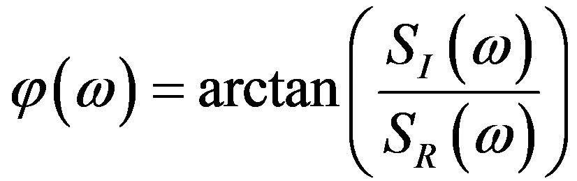
The difficulties in the evaluation of the Fourier Phase Spectrum (FPS) are due to the discontinuities appearing across it. Let  denote the complex Fourier Spectrum of a discrete-time signal
 , obtained via the Discrete-Time Fourier Transform (DTFT). The signal phase is defined as:
 (1)
(1)
where arctan denotes the four quadrant inverse tangent function and ,
,  are the real and imaginary components of
 , respectively.
The FPS suffers from two categories of discontinuities. The first category, called “extrinsic” discontinuities (wrapping ambiguities), is related to the inverse tangent function used in Equation (1); these wrapping ambiguities distort the signal phase content since they are artifacts not related to the signal. To overcome these extrinsic discontinuities and restore the signal phase spectrum, an “unwrapping” algorithm is applied to the FPS [8].
The second category of discontinuities is caused by “intrinsic” characteristics of the signal originating from its nature. These intrinsic discontinuities appear at “critical” frequency points,  , where both the real part and the imaginary part of the Fourier Spectrum
  cross zero simultaneously. Similarly to the extrinsic discontinuities, the intrinsic discontinuities also cause jumps of size
  in the FPS [9,13]. The compensation of the intrinsic discontinuities in the FPS is a two step process: 1) The critical frequency points
  of the signal are detected and 2) the FPS is scanned from lower to higher frequencies; when a critical frequency point
  is met,
  is added or subtracted to all FPS values for
 . Specifically,
  is added [subtracted] to the rest of FPS values if to the frequency point before the critical one corresponds a higher [lower] FPS value.
The methods used to compensate the extrinsic and the intrinsic discontinuities have their drawbacks. Specifically for the compensation of the extrinsic discontinuities, the unwrapping algorithm cannot discriminate between wrapping ambiguities, i.e., extrinsic discontinuities and rapidly changing phase angles caused by structural features of the signal, i.e., intrinsic discontinuities [8]. Conventional unwrapping algorithms compensate all discontinuities blindly as to their respective origins (see also Subsection 5.1). Furthermore for the intrinsic discontinuities compensation method, erroneous critical frequency points  (i.e. intrinsic discontinuities) may be detected due to inaccurate estimation of the zero crossings of the real and the imaginary parts of the Fourier Spectrum because of precision limitations in digital computations [14].
2.2. Implementation of the Phase Spectrum via the z-Transform
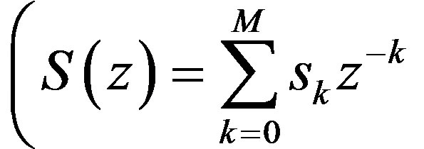
An alternative approach for the removal of the discontinuities appearing in the phase spectrum is based on the ztransform. The phase spectrum of a discrete-time signal  with
with  is constructed in the z-domain by computing and adding the phase contributions of all “zeros” i.e. roots of the polynomial:
 or
or 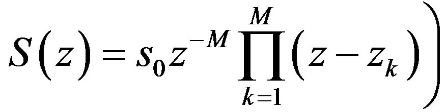
at each frequency point [13]. In the method proposed herein, the roots are evaluated based on the eigenvalues method [15]; moreover, each signal is segmented into frames of 256 samples (i.e. the order of the associated polynomial is M = 255) in order to keep the computational error low (Section 4).
The advantage of this approach is that, unlike the Discrete-Time Fourier Transform (DTFT) approach (Subsection 2.1), it does not exhibit extrinsic discontinuities. Indeed, although the inverse tangent function is still employed for the computation of phase, phase is not wrapped around zero; consequently, wrapping ambiguities do not arise (see Fourier case in Appendix and [7]).
However, the intrinsic discontinuities are still present in this approach and are expressed as “zeros” lying exactly on the circumference of the unit circle in the z-domain. The intrinsic discontinuities should be removed by removing all the “zeros” lying on the circumference of the unit circle and constructing the phase spectrum from the remaining “zeros”. In practice though, due to accuracy limitations in digital computations, one should remove the “zeros” located not only on but also very close to the circumference of the unit circle [9]. For this purpose, a ring is drawn around the circumference of the unit circle and all the “zeros” located within the ring (“sharp zeros”) are removed and the phase spectrum is constructed from the remaining N ≤ M “zeros”:
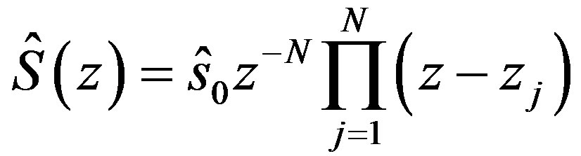 (2)
(2)
The choice of the width of the exclusion ring is a trade-off between information loss (due to the possible removal of useful “zeros”) and the suppression of the intrinsic discontinuities [9] (Subsection 5.1).
2.3. Hartley Magnitude Spectrum and Hartley Phase Spectrum Definitions
The relation between the Fourier Spectrum  and the Hartley Spectrum
  [16], of a signal is given by:
 (3)
(3)
where  and
and  denote the real and the imaginary parts of the Fourier Spectrum, respectively.
Since
 where
where  denotes the Fourier Magnitude Spectrum and
  denotes the FPS (Equation (1)) then,
and
 .
.
Due to the close mathematical relation between the Hartley Spectrum and the Fourier Spectrum, the Hartley Magnitude Spectrum and the Hartley Phase Spectrum are defined following their corresponding Fourier counterparts. Specifically, the definition of the Hartley Magnitude Spectrum follows the definition of the Fourier Magnitude Spectrum [17] and the definition of the Hartley Phase Spectrum or Whitened Hartley Spectrum follows the definition of the Whitened Fourier Spectrum [18-21].
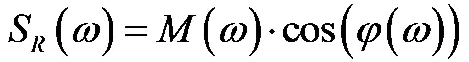
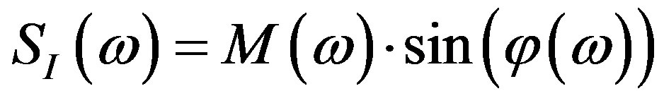
Specifically, along the line of the Fourier Magnitude Spectrum defined as:
 (4)
(4)
where
 the Hartley Magnitude Spectrum is defined as:
 (5)
(5)
where, from Equation (3),
and
 both being real quantities; the absolute value is used in Equation (5) because the product
 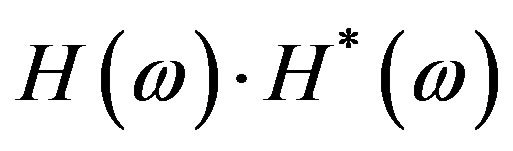 may obtain negative values. Hence, the Hartley Magnitude Spectrum encapsulates magnitude,
  and partially phase,
  , spectral content.
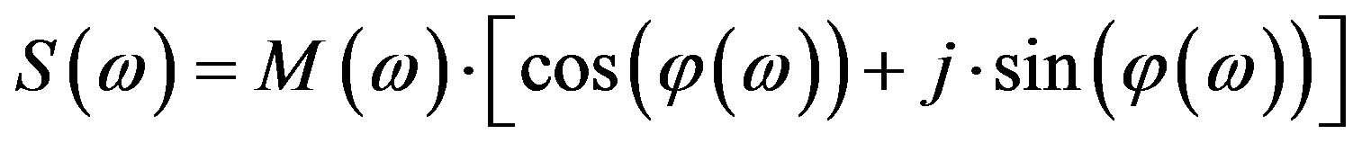
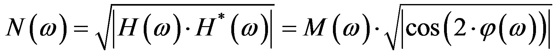
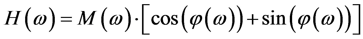
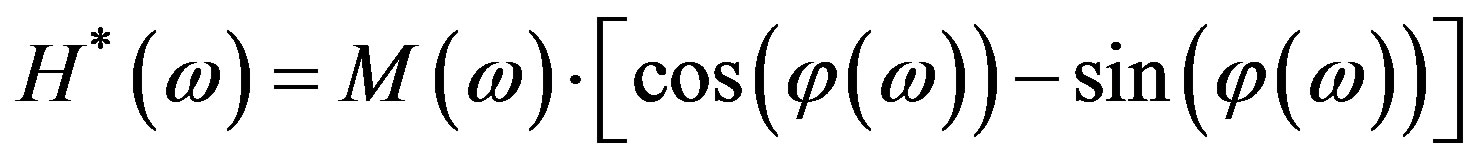
The definition of the Hartley Phase Spectrum (HPS) or Whitened Hartley Spectrum [20], is based on the definition of the Whitened Fourier Spectrum (WFS) which is defined as the ratio of the Fourier Spectrum over the Fourier Magnitude Spectrum—a process known as whitening [19,21]. Hence, the WFS is a complex function that encapsulates the phase content of the signal. The advantage of the WFS over the conventional FPS (Subsection 2.1),  , is that the WFS does not suffer wrapping ambiguities (extrinsic discontinuities). The equivalent whitening process for the Hartley Transform case, called the Whitened Hartley Spectrum, is the ratio of the Hartley Spectrum over the Fourier Magnitude Spectrum. Note that, the Hartley Magnitude Spectrum in Equation (5) is not appropriate for the whitening process, because it conveys partially phase information [20]. Consequently, using Equation (3), the HPS is defined as:
 (6)
(6)
The HPS, being a function of the Fourier Phase , encapsulates the phase content of the signal more efficiently compared with its Fourier counterparts. Specifically, the advantages of the HPS are: (a) It does not suffer from the extrinsic discontinuities that the conventional FPS conveys (Subsection 2.1) and (b) Unlike the WFS, the HPS is a real function; algorithms have been developped in order to compensate its intrinsic discontinuities. In contrast, there is no known method to compensate the intrinsic discontinuities present in the WFS [21].
From Equation (6) it can be seen that the HPS is a function bounded between , a property of practical interest in audio and speech coding applications [20]. Furthermore, the HPS is less sensitive to noise compared with the FPS, due to the form of its probability density function [22].
2.4. Hartley Phase Spectrum Implementation
Two alternative methods are proposed for the implementation of the HPS, in analogy to the methods described in Subsections 2.1 and 2.2 for the FPS.
2.4.1. The Hartley Phase Spectrum via the DTHT
The HPS (Equation (6)), when evaluated in analogy to the method presented in Subsection 2.1 for the FPS, is termed hereafter as the HPS via the Discrete-Time Hartley Transform (DTHT) or . As the inverse tangent function is not employed, no extrinsic discontinuities appear in the HPS; yet, it inherits the same intrinsic discontinuities as the corresponding FPS. The method for the compensation of the intrinsic discontinuities in the
  is similar to the compensation of the intrinsic discontinuities in the FPS via the DTFT. Specifically, for the compensation of an intrinsic discontinuity in the
  appearing in
 , using Equation (6):
 (7a)
(7a)
or
 (7b)
(7b)
Thus, the equivalent of the addition or the subtraction of  in the FPS (intrinsic discontinuity compensation) is the multiplication by -1 for the HPS case, regardless of the HPS value at the frequency point before the critical one. Consequently, the compensation of the intrinsic discontinuities in the HPS proceeds in two steps: 1) The critical points of the signal are detected in the HPS and 2) The HPS is scanned from lower to higher frequencies; whenever a critical frequency point
  is detected, all
  values for
  are multiplied by −1 (a change of sign).
Summarizing, the compensated “FPS via the DTFT” (Subsection 2.1) is obtained in three steps: (a) Evaluation of the FPS using Equation (1); (b) Application of the unwrapping algorithm to the FPS [8]; and (c) Compensation of the intrinsic discontinuities [9].
The compensated “HPS via the DTHT” is obtained in two steps, since it does not suffer extrinsic discontinuities: (a) Evaluation of the HPS using Equation (6); and (b) Compensation of the intrinsic discontinuities.
2.4.2. The Hartley Phase Spectrum via the z-Transform
The second method for the HPS evaluation (see Hartley case in Appendix) is analogous to that of Subsection 2.2 for the FPS. The  thus obtained is termed hereafter as the HPS via the z-transform or
 .
.
3. Statistical Features and Classification
In the experimental part of this work, the feature extraction stage of the pattern recognition process uses selected statistical features, extracted from each spectrogram, to form the feature vectors. The feature vectors are formed using simple rather than sophisticated statistical features because the aim is to compare and then combine the magnitude with the phase spectral information via the same feature extraction process. These features are selected after preliminary experimentation and trials on different alternatives. Each spectrogram (Section 4) is thus represented by an [1 × 8]-sized feature vector, including: The variance, the skewness, the kurtosis, the entropy, the inter-quartile range, the range, the median and the mean absolute deviation [23]. Note that the range is not employed as a feature for the Hartley Phase spectrogram (Section 4), as the latter is limited between  (Equation (6)).
For the audio classification application in particular, the information conveyed by each of the aforementioned statistical features with respect to the magnitude and phase spectrograms is the following: 1) The variance, the inter-quartile range, the mean absolute deviation and the range encapsulate information related to the dynamic range of the spectrum; 2) The skewness and the kurtosis encapsulate the information related to the shape of the spectrum; 3) The median encapsulates the information related to the central level of the spectrum; and 4) The entropy encapsulates the information related to the structural order of the spectrum [24,25].
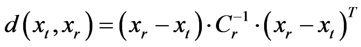
The Mahalanobis distance metric classifier is used for the classification stage of the pattern recognition process. The Mahalanobis distance  between a reference feature vector, xr, and a test feature vector, xt, is given by:
 (8)
(8)
where T denotes transposition and Cr is the covariance matrix of all reference vectors [26].
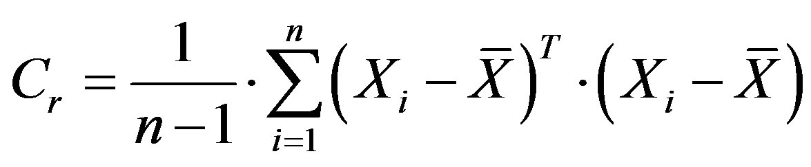
The Mahalanobis distance metric classifier is selected thanks to the normalization capability of the covariance matrix. In alternative classifiers considered, such as the City Block, the Euclidean distance, etc., the degree of variance amongst the values of the feature vectors of the reference data, is not taken into account; consequently, features that have high absolute values dominate the result. Even the standardized Euclidean distance metric classifier, which preserves the variance of each feature vector, does not consider the degree of variance amongst the feature vectors. It should be noted, however, that the accuracy of the results thus obtained is dependent on the accuracy of the Cr estimate available; this in turn depends on the features selected in vector xr and increases with the size of the data set available. The Cr matrix is estimated off-line, by sample averaging, based on the reference set of feature vectors, as:
 (9)
(9)
where n is the number of rows (reference vectors) of an n × m matrix, m is the number of features in each vector (m = 8), Xi is the ith row of the matrix (ith reference vector) and  is the mean row vector across the n columns.
Summarizing, an [1 × 8]-sized reference feature vector is constructed from the mean values of the eight statistical features across each signal in the classifier training set, within each audio class. The Mahalanobis distance is calculated between an incoming test vector and each reference vector; the test vector is assigned to that class whose reference vector is the closest [27].
4. Experimental Procedure
The database used in the experimental part is created based on [28]. It consists of ten different classes of gunshots, namely: 1) Firing a revolver; 2) firing a 0.22 caliber handgun; 3) firing an M-1 rifle; 4) firing a World War II German rifle; 5) firing a cannon; 6) firing a 30-30 rifle, 7) firing a 0.38 caliber semi-automatic pistol; 8) firing a Winchester rifle; 9) firing a 37 mm anti-tank gun; and 10) firing a pistol. These audio recordings are originally stereo (one channel only used here) with 16 bits precision and sampling frequency 44,100 Hz. This database is chosen because all the classes belong acoustically to the same family (fine audio classification—Section 1), thus making the classification task more demanding.
Each one of the ten (10) audio classes consists of ten (10) recordings. Seven of them are used as training data and the rest as test data. For each class, the ten aforementioned recordings (gunshot signals) are manually extracted from a single long waveform provided for the given audio event (class) in the database [28]. In the waveform, the relevant audio event is repeated several times in a sequence (e.g. ten pistol shots). In the cases (classes) where the waveform consists of less than ten repetitions of the signal (gunshots), the additional signals needed to complete the ten samples are created by adding random noise to the original signals extracted from the waveform. Due to the limited number of recordings per class the leave-one-out method of cross-validation is used for the experiments (Section 5).
The type of signal where the gunshots belong is nonstationary transient [29]. Specifically, the gunshot signals belong to the “Meixner” type of transients because they are characterized by their short burst of energy that subsequently decays, [30] Figure 1(a) for class (6) and Figure 1(b) for class (10). Due to the non-stationary nature of the gunshot signals, time-frequency signal representations are required in order to extract the appropriate features for their classification. It is important to mention though that time-frequency distributions, such as the Wigner-Ville distribution, the Wavelet transform, etc., do not utilize the phase content of the signals [31]. Therefore, in the proposed method, features are extracted from distinct magnitude and phase time-frequency distributions in order to encapsulate the non-stationary transient nature of these signals and also to utilize their magnitude and phase content in separate feature vectors.
Specifically, each audio signal is segmented into frames of equal length (256 samples) with zero-padding of the last frame if necessary. This corresponds to an effective window size of 6 msec, which is adequate given the bursty nature of the shots. Each frame is windowed with a Hanning window (no window overlap) and transformed to the frequency domain. The transformed frames are then placed row-wise in a matrix forming a spectrogram. Five different such spectrogram matrices are evaluated for each audio signal, namely:
1. The Fourier Magnitude—based on Equation (4);
2. The Hartley Phase via the z-transform—based on Equation (6) and Subsection 2.4;
3. The Hartley Phase via the DTHT—based on Equation (6) and Subsection 2.4;
4. The Hartley Magnitude—based on Equation (5);
5. The Hartley Transform—based on Equation (3).
The same parameters (frame length, window function) are used for the evaluation of all five spectrograms in order to compare them—in terms of their recognition performance—on the same basis. The conservative frame length of 256 samples helps to keep the computational error of the Hartley Phase via the z-transform spectrogram low (Section 2).
Each of the five aforementioned spectrograms has to be presented to the classifier in a reduced dimensionality form. The statistical features described in Section 3 are extracted from each spectrogram for each audio signal, in order to compress the information of each spectrogram into a compact feature vector.
The recognition performance of the aforementioned spectrograms is compared with the recognition performance of the MFCCs which are features that encapsulate the magnitude content of the signal. Briefly, the MFCCs of a signal are computed as follows: The signal is passed through a pre-emphasis filter (a typical first order filter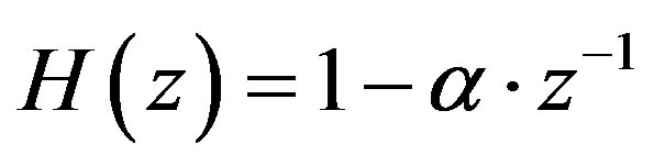 ,
,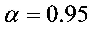 ) in order to become spectrally flat and amplify areas of its spectrum that are critical to hearing. After windowing, the Fourier Transform is applied to each frame of the signal and the absolute magnitude spectrum is evaluated. The linear frequency axis (f) of the magnitude spectrum is then warped into the Melscale frequency axis (mel) defined as:
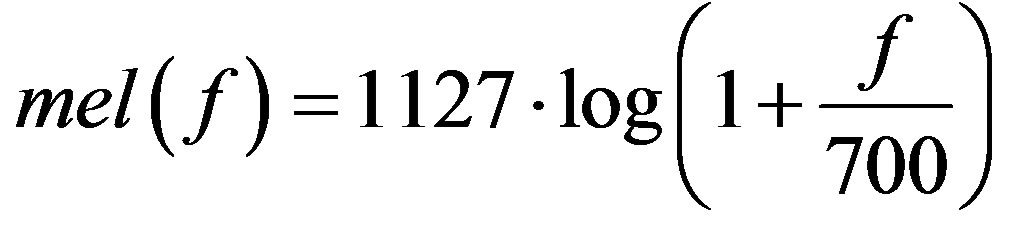
where log denotes logarithm. The warped magnitude spectrum is passed through a bank of triangular-shaped filters that are linearly spaced in the 0 Hz to 1000 Hz range whereas above this, their central frequencies are given by: 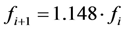 where the first central frequency, f1, equals to 1 kHz. Subsequently, for each frame, the logarithmic function is used to compress the dynamic range of the magnitude spectral values and the Discrete Cosine Transform is applied to the logarithm of the magnitude of the filter-bank outputs [12]. A defined number of the first MFCCs (excluding the 0th coefficient) are retained from each frame and a matrix is formed (e.g., 20 coefficients × 80 frames). The mean value of each MFCC is calculated per frame in order to form the feature vector (e.g. for the aforementioned example, the size of the feature vector is 20 × 1). Finally, via its MFCC feature vector, each signal is classified to the corresponding class based on the Mahalanobis distance metric classifier. Hence, in the following sections, the spectrogram-based feature extraction method, proposed here, is compared with the MFCC-based method on a fair comparison basis.
4.1. Spectrogram Selection and Preliminary Classification Results
The first set of classification experiments addresses the ten audio classes classification task and uses each of the five aforementioned spectrograms as an individual “expert”. Classification scores are presented in Table 1. Note that no discontinuities compensation or removal is employed for the phase-related spectrograms (see also Subsection 5.1).
As it can be observed from Table 1, the Fourier Magnitude spectrogram yields the highest classification rate (66.7%); this indicates that it encapsulates the signal information content more efficiently than the rest of the spectrograms. A closer examination of the classification results, however, reveals that there are certain audio classes (namely, classes: (2), (4), (5) and (10)) where the Fourier Magnitude spectrogram “expert” yields significantly reduced scores that draw the Fourier Magnitude spectrogram average down to 66.7%. This prompts further investigation as to the features that would be more appropriate for those “hard” classes.
In view of the above observation, for the next set of experiments, the five spectrograms are grouped in three categories based on the information they convey. On the basis of this categorization, two alternative experiments
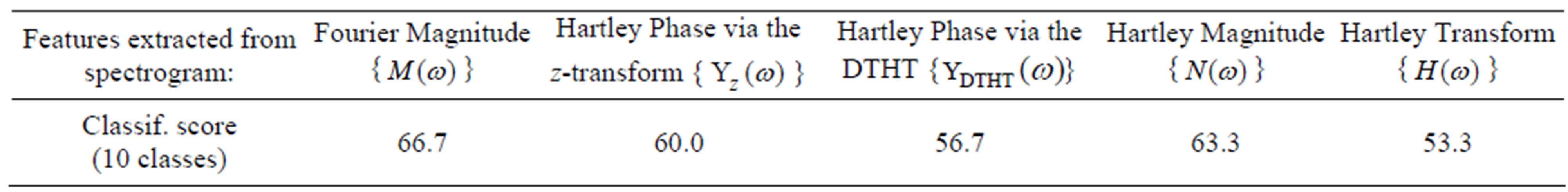
Table 1. Correct classification rates (%) for individual spectrograms.
are carried out, where one spectrogram is selected from each of the three categories. These experiments aim tocompare the classification performance when spectrograms of the three aforementioned categories are combined with the case where only magnitude-related features are used (Fourier Magnitude spectrogram and MFCCs). Specifically, the three categories are:
Category 1—Spectrograms that encapsulate magnitude content: The Fourier Magnitude spectrogram preserves only the magnitude content of the signal.
Category 2—Spectrograms that encapsulate phase content: The Hartley Phase via the z-transform spectrogram and the Hartley Phase via the DTHT spectrogram belong to this category. The Hartley Phase via the z-trans form offers the advantage of the flexible method for the removal of the intrinsic discontinuities using the “zeros” exclusion ring (Subsections 2.2 and 2.4), while the Hartley Phase via the DTHT relies on the compensation rather than the removal of the intrinsic discontinuities (Subsection 2.4). The Hartley Phase via the DTHT avoids the empirical decision on the exclusion ring width; yet, the choice of this very parameter offers to the Hartley Phase via the z-transform the flexibility to control the degree of reduction of the intrinsic discontinuities at the risk of increasing information loss (Subsection 5.1). Clearly, the two approaches are not equivalent; however, since their recognition performance is comparable (60.0% versus 56.7% in Table 1) both the Hartley Phase via the z-transform and the Hartley Phase via the DTHT spectrograms are used for the experiments.
Category 3—Spectrograms that encapsulate a combination of magnitude and phase contents:
The Hartley Magnitude (contains partially phase information, Subsection 2.3) and the Hartley Transform spectrograms belong to this category. The Hartley Transform spectrogram obtains a 10.0% lower classification rate compared with the Hartley Magnitude spectrogram (Table 1); hence, the Hartley Magnitude spectrogram is selected for the experiments.
Thus, Experiment 1 combines: (a) The Fourier Magnitude spectrogram (Category 1); (b) The Hartley Phase via the DTHT spectrogram (Category 2); and (c) The Hartley Magnitude spectrogram (Category 3) while Experiment 2 combines: (a) The Fourier Magnitude spectrogram (Category 1); (b) The Hartley Phase via the ztransform spectrogram (Category 2); and (c) the Hartley Magnitude spectrogram (Category 3).
The three independent “experts” (spectrograms), used in each experiment, are combined in order to produce the final classification decision based on the majority vote rule. For each audio signal three feature vectors are formed, one for each of the three aforementioned spectrograms. In distance metric classification, a signal is classified to a certain class based on the minimum distance between the test and the reference feature vectors (Section 3). Hence, in this case, if two or three out of the three “experts” agree then, the audio signal is classified to this class. In case of a tie, the decision is taken based on the class proposed by the Fourier Magnitude spectrogram “expert”.
The classification scores of Experiment 1 and Experiment 2 are compared with the classification score obtained based on the MFCCs. These results aim to compare the proposed feature extraction method that combines magnitude with phase information (Experiments 1 and 2) with features that encapsulate efficiently only the magnitude content of the signal.
A series of preliminary experiments is carried out in order to specify the parameters of the MFCC algorithm with respect to the recognition performance. The highest classification rate is obtained when the signal frame size is 1024 samples, using a Hanning window, 32 filters in the filter bank and a frame increment of 512 samples. For these parameters, further experiments are conducted so as to determine the number of MFCCs (i.e. size of feature vector) that provides the highest classification score. Specifically, the number of coefficients tested ranges from 4 to 32 in steps of 2. The classification rate increases with the number of coefficients reaching the highest rate (73.3%) when the number of coefficients retained is 20; beyond this order the rate decreases. Representative classification rates are provided in Table 2.
Since the MFCCs encapsulate purely the magnitude content of the signal, their recognition performance is similar to the Fourier Magnitude spectrogram; therefore, as expected, they also yield considerably reduced scores for the same four audio Classes (2), (4), (5) and (10).
However, for the ten classes the classification rate obtained based on the Fourier Magnitude spectrogram (Table 1) is lower compared with the MFCCs (Table 2), due to the significant compression qualities of the latter.
The classification results obtained from Experiments 1and 2 are presented and compared with the classification rates of the MFCCs, in Subsection 5.2 and Table 3.
5. Classification Results and Discussion
5.1. Hartley Phase Spectrograms and Recognition Performance
For the two cases of the Hartley Phase spectrograms (computation via the DTHT and via the z-transform), the spectrogram matrices are replaced by matrices formed by evaluating the first order discrete difference along each
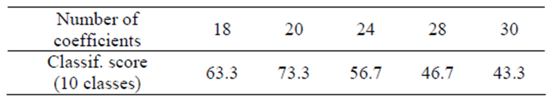
Table 2. Correct classification rates (%) for the MFCC features.
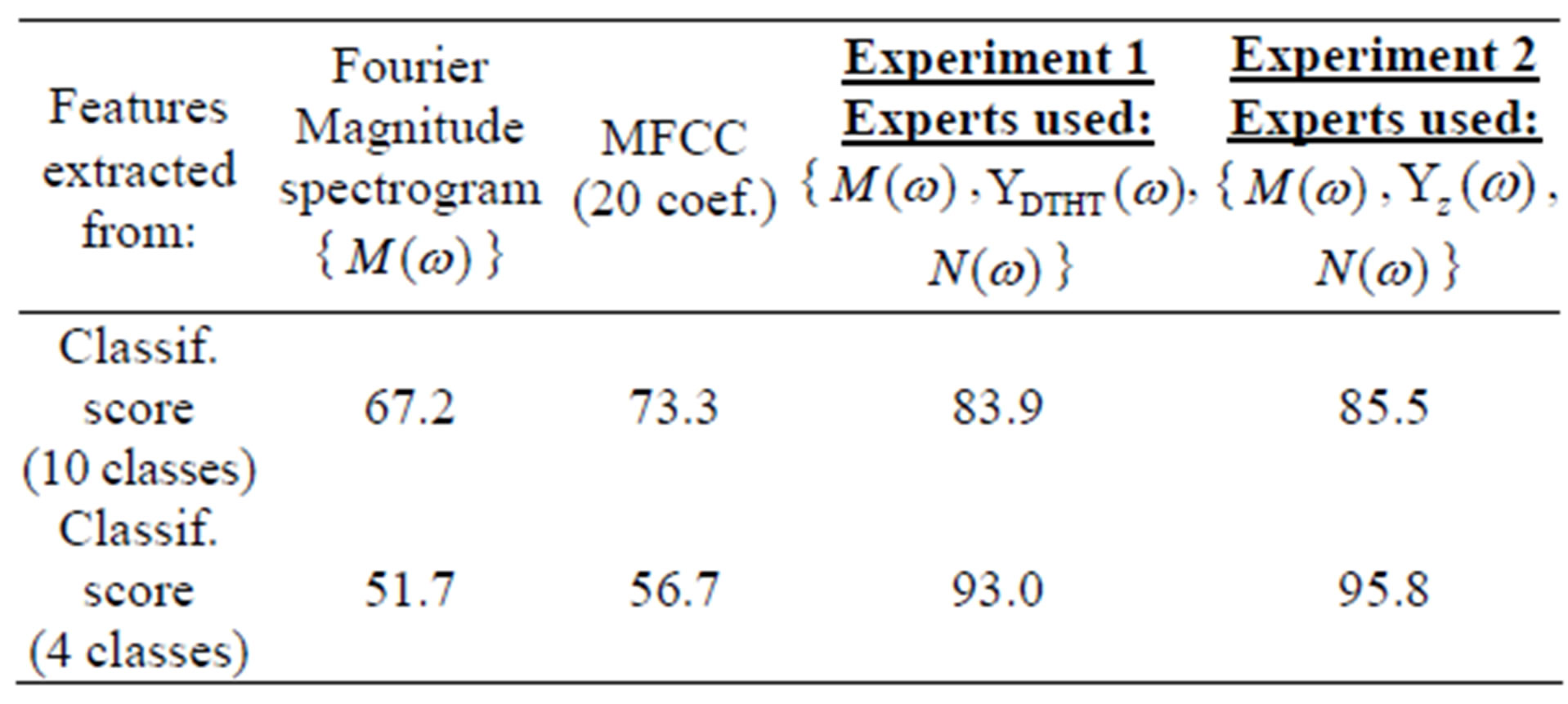
Table 3. Correct classification rates (%) for Fourier Magnitude spectrogram, MFCC, Experiments 1 & 2.
row of the original matrices. The feature vectors are then extracted from these phase difference matrices. Experiments on the audio signals database yield a classification rate improvement of 14.0% on average when using the first order discrete difference of the Hartley Phase spectrograms (via the DTHT and via the z-transform) over the case where the phase difference is not utilized.
Similarly, a classification rate improvement of 16.7% on average is observed when the phase difference is applied to the Fourier Phase spectrograms (via the DTFT and via the z-transform). This recognition performance improvement is in agreement with results reported in [32], where it is claimed that the phase difference is less affected by noise than the phase per se. This observation indicates that for signals such as the gunshots, which are characterized by their considerable noise content, the derivative (first order difference) of the phase spectrum— which encapsulates the information related to the velocity with which each frequency “travels” within the signal—is a more informative feature for classification compared with the phase spectrum. The classification rates of the Hartley Phase via the z-transform and the Hartley Phase via the DTHT spectrograms presented in Tables 1 and 3 (Experiments 1 & 2) as well as all the classification rates of the Hartley Phase and the Fourier Phase spectrograms presented in this work are obtained by evaluating the first order discrete difference. In case the classification results are obtained when the discontinuities are compensated or removed from the Hartley Phase and the Fourier Phase spectrograms, the first order discrete difference is evaluated after the compensation or removal of the discontinuities.
Hartley Phase via the DTHT Spectrogram The classification rate, averaged across all ten audio classes, obtained using the Hartley Phase via the DTHT spectrogram when the intrinsic discontinuities are compensated (no extrinsic discontinuities exist in the HPS, Subsection 2.4) is 81.6% whereas, the classification rate obtained when the discontinuities are not compensated is 56.7% (Table 1). Similarly, for the Fourier Phase via the DTFT spectrogram the highest classification score (71.4%) is obtained when both the extrinsic and the intrinsic discontinuities are compensated.
The classification scores obtained using the Hartley Phase via the DTHT versus the Fourier Phase via the DTFT spectrograms are summarized in three cases:
1) When both spectrograms are employed without any type of compensation, the Hartley Phase spectrogram classification score of 56.7% (Table 1) outperforms the Fourier Phase spectrogram classification score of 43.3%, while2) When both spectrograms contain only intrinsic discontinuities, i.e. after extrinsic discontinuities are compensated in the Fourier Phase spectrogram then, the Fourier Phase spectrogram classification score of 66.7% outperforms the Hartley Phase spectrogram score of 56.7% (Table 1). Finally3) When both spectrograms are processed to compensate the intrinsic discontinuities, the Hartley Phase spectrogram (intrinsic discontinuities compensated) score of 81.6% outperforms the Fourier Phase spectrogram (extrinsic and intrinsic discontinuities compensated) score of 71.4%.
The counter-intuitive behavior of the Fourier Phase spectrogram performance to exceed the Hartley Phase spectrogram performance in Case (2) is due to the fact that while compensating extrinsic discontinuities from the FPS, a number of intrinsic discontinuities is inevitably also compensated, due to the “blind” compensation behavior of the unwrapping algorithm. Specifically, the unwrapping algorithm adds multiples of  in case a phase jump equal to or greater than
  occurs in the FPS and hence in theory, the unwrapping algorithm should simultaneously compensate both the extrinsic and the intrinsic discontinuities, since the intrinsic discontinuities also cause phase jumps of
  in the FPS (Subsection 2.1). However, in many cases due to computational inaccuracies the intrinsic discontinuities appearing in the FPS cause phase jumps that are marginally less than
 . Therefore in practice, the unwrapping algorithm compensates the extrinsic discontinuities and also a certain number of the intrinsic discontinuities, a fact which explains the higher classification rate of the Fourier Phase spectrogram, since the recognition performance is related to the existence of discontinuities in the phase spectrum.
However, of practical interest for further processing steps is the Case (3) situation, where all discontinuities are compensated and the Hartley Phase via the DTHT spectrogram shows a clear advantage.
Moreover, for the classification rates of Case (3) and for the classification rates of the Hartley Phase via the z-transform spectrogram when discontinuities are removed (i.e. cases of non-zero width exclusion ring) that is described in the following paragraph, the leave-oneout method of cross-validation, [27], is employed due to the limited number of signals available within each audio class (ten signals per class). For the classification results of the Fourier Magnitude spectrogram and Experiments 1 and 2, which are presented in Subsection 5.2 and Table 3, the leave-one-out method is also employed. In contrast, the leave-one-out method is not employed in the preliminary experiments of Table 1 (individual “experts”). This explains the slightly different scores in the Fourier Magnitude spectrogram “expert” between Tables 1 (66.7%) and 3 (67.2%).
Hartley Phase via the z-Transform Spectrogram The removal of the “sharp zeros” using the exclusion ring reduces the discontinuities in the HPS (Subsections 2.2 and 2.4). However, as the ring width increases the number of “zeros” excluded also increases, thus causing information loss.
Hence, for the classification experiments the ring width is varied from zero (i.e. no intrinsic discontinuities removed) to 0.001 (15.0% of the signal “zeros” excluded on average), with a step of 0.00001. Further increase of the ring width would risk unreliable results, due to the limited number of “zeros” used for the evaluation of the phase spectrum.
The experimental results, using the audio database, show that the classification rate obtained from the Hartley Phase via the z-transform spectrogram for a zero ring width is 60.0% (Table 1). The classification rate increases as the ring width increases reaching its highest value (83.7%) for a ring width equal to 0.00003 (on average 1.0% of the “zeros” are excluded). However, as the ring width further increases from 0.00004 to 0.001, the classification rate gradually decreases becoming 65.3% for the widest ring width tested (0.001). For the Fourier Phase via the z-transform spectrogram the same ring width as in its Hartley counterpart has provided the highest classification rate.
The classification rate obtained from the Hartley Phase via the DTHT spectrogram when the discontinuities are compensated is 10.2% higher compared with its Fourier counterpart and similarly, the classification rate obtained from the Hartley Phase via the z-transform spectrogram is 4.1% higher (average over all the ring widths tested) compared with its Fourier counterpart. These results indicate that the phase spectral content is presented to the classifier in an improved manner using the HPS as compared with the FPS.
5.2. Classification Results of the Combinatory Scheme
As mentioned in Subsection 4.1, the classification rate obtained based on the magnitude feature vectors extracted from the Fourier Magnitude spectrogram and the MFCCs, drops considerably for certain classes of audio signals—namely, for Classes (2), (4), (5) and (10). Consequently, improvement of recognition performance is sought through the use of features extracted from the phase spectrograms. The classification rates obtained from Experiments 1 and 2 (Subsection 4.1) are compared with the classification rates obtained from the Fourier Magnitude spectrogram and the MFCCs in order to test whether the combination of magnitude with phase related features is beneficial compared with the use of purely magnitude related features.
In the first [second] row of Table 3 are presented the classification rates for the ten classes [four “hard” classes]. For the case of the ten classes, the recognition rate is increased from 67.2% obtained from the Fourier Magnitude spectrogram to 83.9% (Experiment 1) and 85.5% (Experiment 2) obtained from the combinatory scheme, due to the inclusion of the phase related features. More importantly, the recognition improvement is much more pronounced for the case of the four “hard” classes. Indeed, the classification score is increased from 51.7% using the Fourier Magnitude spectrogram to 93.0% (Experiment 1) and 95.8% (Experiment 2) using the combinatory scheme; for these four classes and for both Experiments 1 and 2, the classification improvement is significant at level 0.95 based on the statistical matchedpairs t-test performed here, along the line of [33] for speech. For Experiment 2 (Table 3), where the Hartley Phase via the z-transform spectrogram is used as one out of the three spectrograms (Subsection 4.1), the classification rates presented are obtained when the ring width is set to its experimentally optimal value of 0.00003 (Subsection 5.1). However, it is important to report that for the four classes case in Experiment 2, the classification rate improvement is still significant at level 0.95 even when the ring width is set to zero.
Similarly to the Fourier Magnitude spectrogram, the MFCCs yield lower classification rates compared with the combinatory scheme (Experiments 1 and 2). Specifically, for the ten classes case the classification rate obtained via the MFCCs is 73.3% and for the four classes case the classification rate is 56.7% (Table 3).
6. Conclusions
The usefulness of phase as an assistive frequency domain feature for audio classification applications is argued in this work. An audio database with gunshot signals bearing considerable spectral magnitude similarities is selected as a demanding test case.
The experimental results show that the classification rate of the combinatory scheme, which encapsulates both the magnitude and the phase spectral content of the signal, is higher compared with the rate obtained from purely magnitude spectral features such as the Fourier Magnitude Spectrum or the MFCCs. Specifically, the recognition rate of the combinatory scheme is 41.3% and 44.1% higher for the four “hard” classes in Experiments 1 and 2 in Table 3, respectively, as compared with the use of the Fourier Magnitude spectrogram only. Moreover, the same rates are 36.3% and 39.1% higher for the four “hard” classes in Experiments 1 and 2 in Table 3, respectively, as compared with the use of the MFCCs only. It is important to mention that similar conclusions are drawn from the classification results obtained from speech rather than audio signals [17]. It is also important that the higher classification rates obtained when phase spectral features are combined with magnitude spectral features have been observed uniformly across all the experiments carried out here.
Furthermore, the classification results indicate that the Hartley Phase Spectrum (or Whitened Hartley Spectrum) encapsulates the phase content of the signal more efficiently than the conventional Fourier Phase Spectrum; the recognition rates of the Hartley Phase via the DTHT spectrogram and the Hartley Phase via the z-transform spectrogram are 10.2% and 4.1% higher compared to their Fourier counterparts, respectively (Section 5). The Hartley Phase Spectrum suffers fewer discontinuities, is more tolerant to noise and it is easier to process compared to the Fourier Phase Spectrum.
The encouraging results obtained experimentally from the specific audio database are indicative of the potential of the proposed combined use of phase and magnitude based features for audio classification tasks. However, further research is necessary in order to investigate the generalization ability of the proposed approach when applied to audio signals of classes other than shots or bursts; yet, bearing spectral magnitude similarities. Real time conditions constitute an additional challenge towards which further research may be conducted.
The proposed method may also be applied in two-dimensional signal (image) processing, where the signal phase is already being recognized as an important feature. Specifically, it would be worth to investigate whether the properties of the Hartley Phase Spectrum offer a relative advantage in image processing applications such as Synthetic Aperture Radar (SAR) or Magnetic Resonance Imaging (MRI).
7. Acknowledgements
Research co-funded by the E.U. (European Social Fund) and national funds, action “Archimedes III— Funding of research groups in T.E.I.”, under the Operational Programme “Education and Lifelong Learning 2007-2013”.

REFERENCES
- L. D. Alsteris and K. K. Paliwal, “Short-Time Phase Spectrum in Speech Processing: A Review and Some Experimental Results,” Digital Signal Processing, Vol. 17, No. 3, 2007, pp. 578-616. doi:10.1016/j.dsp.2006.06.007
- P. Aarabi, G. Shi, M. M. Shanechi and S. A. Rabi, “PhaseBased Speech Processing,” World Scientific Publishing Co. Pte Ltd., Singapore Cigy, 2006.
- D. Eck and N. Casagrande, “Finding Meter in Music Using an Autocorrelation Phase Matrix and Shannon Entropy,” Proceedings of the 6th International Conference on Music Information Retrieval (ISMIR 2005), London, 11-15 September 2005, pp. 504-509.
- E. Cano, G. Schuller and C. Dittmar, “Exploring Phase Information in Sound Source Separation Applications,” Proceedings of the 13th International Conference on Digital Audio Effects (DAFx-10), Graz, 6-10 September 2010, pp. 1-7.
- F. Jin, S. Krishnan and F. Sattar, “Adventitious Sounds Identification and Extraction Using Temporal-Spectral Dominance-Based Features,” IEEE Transactions on Biomedical Engineering, Vol. 58, No. 11, 2011, pp. 3078- 3087.
- R. M. Hegde, H. A. Murthy and V. R. R. Gadde, “Significance of the Modified Group Delay Feature in Speech Recognition,” IEEE Transactions on Audio, Speech, and Language Processing, Vol. 15, No. 1, 2007, pp. 190-202. doi:10.1109/TASL.2006.876858
- B. Bozkurt, L. Couvreur and T. Dutoit, “Chirp Group Delay Analysis of Speech Signals,” Speech Communication, Vol. 49, No. 3, 2007, pp. 159-176. doi:10.1016/j.specom.2006.12.004
- J. M. Tribolet, “A New Phase Unwrapping Algorithm,” IEEE Transactions on Acoustics, Speech and Signal Processing, Vol. 25, No. 2, 1977, pp. 170-177. doi:10.1109/TASSP.1977.1162923
- H. Al-Nashi, “Phase Unwrapping of Digital Signals,” IEEE Transactions on Acoustics, Speech and Audio Processing, Vol. 37, No. 11, 1989, pp. 1693-1702. doi:10.1109/29.46552
- I. Paraskevas and E. Chilton, “Combination of Magnitude and Phase Statistical Features for Audio Classification,” Acoustics Research Letters Online, Vol. 5, No. 3, 2004, pp. 111-117. http://asadl.org/arlo/resource/1/arlofj/v5/i3/p111_s1?bypassSSO=1 doi:10.1121/1.1755731
- Y. Wang, Z. Liu and J.-C. Huang, “Multimedia Content Analysis Using both Audio and Visual Cues,” IEEE Signal Processing Magazine, Vol. 17, No. 6, 2000, pp. 12-36. doi:10.1109/79.888862
- S. Davis and P. Mermelstein, “Comparison of Parametric Representations for Monosyllabic Word Recognition in Continuously Spoken Sentences,” IEEE Transactions on Acoustics, Speech and Signal Processing, Vol. 28, No. 4, 1980, pp. 357-366. doi:10.1109/TASSP.1980.1163420
- J. G. Proakis and D. G. Manolakis, “Digital Signal Processing Principles, Algorithms, and Applications,” Macmillan Publishing Company, New York, 1992.
- G. E. Forsythe, M. A. Malcom and C. B. Moler, “Computer Methods for Mathematical Computations,” Prentice-Hall, Upper Saddle River, 1977.
- G. A. Sitton, C. S. Burrus, J. W. Fox and S. Treitel, “Factoring Very-High-Degree Polynomials,” IEEE Signal Processing Magazine, Vol. 20, No. 6, 2003, pp. 27-42. doi:10.1109/MSP.2003.1253552
- R. N. Bracewell, “The Fourier Transform and Its Applications,” McGraw-Hill Book Company, New York, 1986.
- I. Paraskevas and M. Rangoussi, “The Hartley Phase Spectrum as an Assistive Feature for Classification,” Advances in Nonlinear Speech Processing, Springer Lecture Notes in Computer Science, Vol. 5933, 2010, pp. 51-59.
- I. Paraskevas and M. Rangoussi, “The Hartley Phase Cepstrum as a Tool for Improved Phase Estimation,” Proceedings of the 16th International Conference on Systems, Signals and Image Processing (IWSSIP 2009), Chalkida, 18-20 June 2009, pp. 1-4. doi:10.1109/IWSSIP.2009.5367774
- I. Moreno, V. Kober, V. Lashin, J. Campos, L. P. Yaroslavsky and M. J. Yzuel, “Color Pattern Recognition with Circular Component Whitening,” Optics Letters, Vol. 21, No. 7, 1996, pp. 498-500. doi:10.1364/OL.21.000498
- E. Chilton, “An 8kb/s Speech Coder Based on the Hartley Transform,” Proceedings of the ICCS ‘90 Communication Systems: Towards Global Integration, Singapore, 5-9 November 1990, Vol. 1, pp. 13.5.1-13.5.5.
- I. Paraskevas and M. Rangoussi, “The Hartley Phase Cepstrum as a Tool for Signal Analysis,” Advances in Nonlinear Speech Processing, Springer Lecture Notes in Computer Science, Vol. 4885, 2007, pp. 204-212.
- I. Paraskevas and M. Rangoussi, “The Hartley Phase Spectrum as a Noise-Robust Feature in Speech Analysis,” Proceedings of the ISCA Tutorial and Research Workshop (ITRW) on Speech Analysis and Processing for Knowledge Discovery, Aalborg, 4-6 June 2008.
- A. Papoulis, “Probability and Statistics,” Prentice-Hall, Inc., Upper Saddle River, 1990.
- T. Lambrou, P. Kudumakis, R. Speller, M. Sandler and A. Linney, “Classification of Audio Signals Using Statistical Features on Time and Wavelet Transform Domains,” Proceedings of the IEEE International Conference on Acoustics, Speech, and Signal Processing (ICASSP 1998), Seattle, 12-15 May 1998, Vol. 6, pp. 3621-3624.
- S. Theodoridis and K. Koutroumbas, “Pattern Recognition,” Academic Press, San Diego, 1999.
- P. C. Mahalanobis, “On the Generalized Distance in Statistics,” Proceedings of the National Institute of Science of India, Vol. 2, No. 1, 1936, pp. 49-55.
- R. O. Duda, P. E. Hart and D. G. Stork, “Pattern Classification,” 2nd Edition, John Wiley & Sons, Hoboken, 2000.
- Audio Database, “505 Digital Sound Effects, (Disk 3/5: 101 Sounds of the Machines of War),” Delta Entertainment Corporation, Santa Monica, 1993.
- M. R. Azimi-Sadjadi, Y. Jiang and S. Srinivasan, “Acoustic Classification of Battlefield Transient Events Using Wavelet Sub-Band Features,” SPIE Proceedings, Vol. 6562, 2007, Article ID: 656215. doi:10.1117/12.722296
- E. G. P. Schuijers, A. W. J. Oomen, A. C. den Brinker and A. J. Gerrits, “Advances in Parametric Coding for High-Quality Audio,” Proceedings of the 1st IEEE Benelux Workshop on Model based Processing and Coding of Audio (MPCA 2002), Leuven, 15 November 2002, pp. 73-79.
- J. Jinshui, C. Hao, L. Bin and S. Perming, “Research on the Method of Features Extraction for Non-Stationary Transient Signal Based on EMD Method,” Proceedings of the International Conference on Communication Software and Networks (ICCSN 2009), Macau, 27-28 February 2009, pp. 637-641.
- P. Gough, “A Particular Example of Phase Unwrapping Using Noisy Experimental Data,” IEEE Transactions on Acoustics, Speech, and Signal Processing, Vol. 31, No. 3, 1983, pp. 742-744. doi:10.1109/TASSP.1983.1164099
- L. Gillick and S. J. Cox, “Some Statistical Issues in the Comparison of Speech Recognition Algorithms,” Proceedings of the IEEE International Conference on Acoustics, Speech, and Signal Processing (ICASSP 1989), Glasgow, 23-26 May 1989, Vol. 1, pp. 532-535.
Appendix
The phase contribution of a single “zero”, z, to a given frequency point ω (point C on the unit circle, in Figure 2) equals:
• For the Fourier case, based on Equation (1),
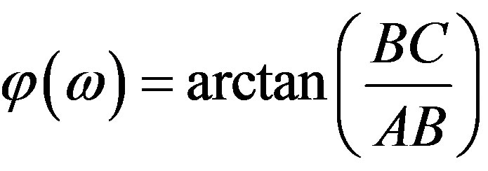 , and
, and
• For the Hartley case, based on Equation (6),
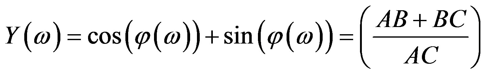 .
.
Furthermore, in case there exist L “zeros” on the z-plane then, their phase contribution to a given frequency point ω, is:
• For the Fourier case, [13],
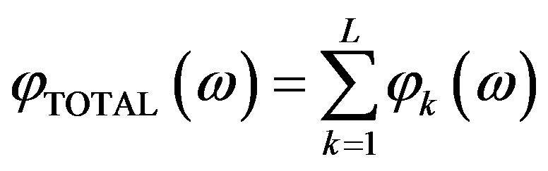 and
and
• For the Hartley case,
 .
.
This process has to be repeated for all the frequency points of interest, in order to evaluate the FPS or the HPS.
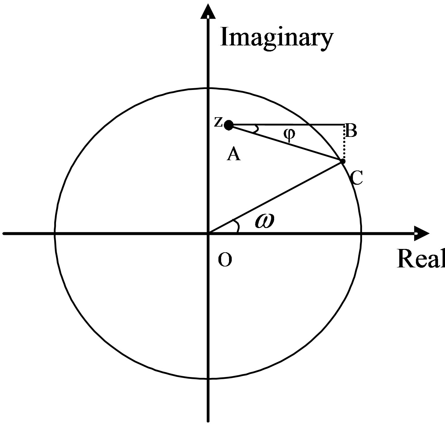
Figure 2. Geometric interpretation of the phase contribution of a single “zero”, z, on the z-plane to a given frequency point ω (point C on the unit circle).