Journal of Mathematical Finance
Vol.3 No.1A(2013), Article ID:29343,9 pages DOI:10.4236/jmf.2013.31A018
Exploiting Market Integration for Pure Alpha Investments via Probabilistic Principal Factors Analysis
1Eonos Investment Technologies, Paris, France
2University of Evry-Val-d’Essone, Evry, France
3Axianta Research, Nicosia, Cyprus
Email: geotzag@gmail.com, juliana@eonos.com, dplsthomas@gmail.com
Received January 3, 2013; revised February 8, 2013; accepted February 19, 2013
Keywords: Market Integration; Risk budgeting; Probabilistic Principal Component Analysis
ABSTRACT
In this paper, a long-short beta neutral portfolio strategy is proposed based on earnings yields forecasts, where positions are modified by accounting for time-varying risk budgeting by employing an appropriate integration measure. In contrast to previous works, which primarily rely on a standard principal component analysis (PCA), here we exploit the advantages of a probabilistic PCA (PPCA) framework to extract the factors to be used for designing an efficient integration measure, as well as relating these factors to an asset-pricing model. Our experimental evaluation with a dataset of 12 developed equity market indexes reveals certain improvements of our proposed approach, in terms of an increased representation capability of the underlying principal factors, along with an increased robustness to noisy and/or missing data in the original dataset.
1. Introduction
Markets constitute a highly dynamically evolving universe, which undergoes through distinct time periods, and reacts in diverse conditions and phenomena, thus, monitoring the opportunities which appear for investors during these periods is of significant importance. An approach to take this behavior into account in asset management is to exploit the importance of the market factor to explain expected returns. More specifically, the part of the variance related to the global market component of risk can be considered as a proxy of market integration. In this context, integration implies that all barriers are eliminated and therefore risk premia associated with global factors are identical in any of such markets.
Construction of optimal portfolios by accounting not only for the diversification across assets, but also across time, attracted the interest of the research community during the last decades [1-4]. In a recent work [5], an alternative way of taking the time-varying risk aversion of the investor into account was proposed. More specifically, a simple and easily implemented two-stage process was introduced, where optimal weights are determined first by suitable optimization techniques and then the weights are adjusted according to a suitable integration measure.
By adopting the same assumptions as in [5], based on the capital asset-pricing model (CAPM) [6], a portfolio can be decomposed in two individual components, namely, the beta component and the alpha component. The beta component corresponds to the part exposed to market risk, while here we consider alpha as the portfolio’s return generated by a risk exposure unrelated to the market risk, where the market portfolio is an international portfolio. A pure alpha strategy is employed, which is not related to the market risk.
The developed strategy is based on the intuition that if global factors determine strongly the excess returns, then less alpha opportunities are left for long-short investors. It is then straightforward to use market integration as a guide for risk-budgeting decisions. Indeed, one would expect that an investment manager would allocate more risk to those decisions that he is most confidence in, rather than to those he feels less certain about.
The standard principal component analysis (PCA) was employed in [5] as a method to construct a measure of integration based on the average percentage of variance explained by the first principal factor. However, the standard PCA approach may suffer from several drawbacks, such as, the sensitivity to outliers, the inaccuracy in case of noisy data, or when the original data are corrupted with missing values. In this study, we overcome these limitations by measuring integration in the framework of probabilistic PCA (PPCA) [7]. More specifically, the principal factors are extracted based on an associated probabilistic model for the observed data, as well as for the potential noise which may corrupt the data. Then, a simple correlation-based integration measure is employed, which is related to the market risk component, while being highly robust in case of noisy data and/or missing values in the original time-series. In addition, this process is carried out in overlapping time-windows to manage risk through time, in conjunction with an adaptation of our long-short weights at each date in a way such that when markets are strongly integrated, a more conservative position is taken, thus, protecting our strategy from the risk we would face during periods of high integration, when markets tend to exhibit a strong directional trend.
The rest of the paper is organized as follows: Section 2 introduces the main principles of PPCA and analyzes in detail the proposed methodology for portfolio optimization. In Section 3, an experimental evaluation of the proposed approach is performed on a set of 14 developed equity markets, while Section 4 concludes and gives directions for further extensions.
2. Market Integration via PPCA
Market integration is a fundamental concept in financial economics [8,9]. Especially for investors, integration would provide a broader range of available assets and lower risk premia, but at the cost of fewer diversification opportunities. Markets are internationally integrated if the reward for risk is identical regardless the market one trades in. Previous works [10,11] exploited an increase in the common component of equity returns data as an indication of higher integration, although such approaches do not measure market integration in the strict sense.
Motivated by [12], where several distinct measures of market co-movements were analyzed, a simple, though still efficient, integration measure is designed by extracting the main factors explaining the cross-sectional equity returns in terms of the average percentage of variance explained by the first significant principal components. However, the performance of the standard PCA may deteriorate in several cases, such as, the presence of a noisy behavior in the original data, and/or the case where a portion of the original data values may be missing or we don’t have access to. The recently introduced framework of PPCA [7] is capable of overcoming such limitations, and it is exploited in our proposed market integration measure to build portfolios for pure alpha investors.
2.1. Linear Multiple Factor Structure
In the subsequent analysis, we consider an ensemble of M time-series  each one with N observations representing equity returns. This ensemble is assumed to follow a linear multiple factor structure, as follows:
 (1)
(1)
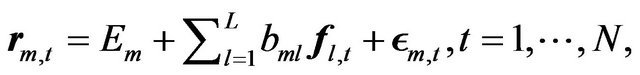
where L is the number of common factors, which capture the systematic component of risk, denotes the expected return on the m-th asset,
  is the realization at time t of the l-th common factor,
  is the sensitivity of the m-th asset to the movements of the l-th factor, and
  denotes the noise term. The assumption for a linear multiple factor structure yields that the factors can be estimated by employing a principal component analysis, in our case working in a probabilistic framework.
2.2. Probabilistic PCA
In this section, the main principles of PPCA are introduced in brief. A remarkable feature of the typical PCA is the absence of an associated probabilistic model for the observed data. A probabilistic formulation of PCA is obtained from a Gaussian latent-variable model, with the principal axes emerging as maximum-likelihood (ML) estimates. Moreover, the latent-variable formulation results naturally in an iterative, and computationally efficient, expectation-maximization (EM) algorithm for performing PPCA.
A further motivation is that PPCA is characterized by some additional practical advantages: a) the probabilistic model offers the potential to extend the scope of standard PCA. For instance, multiple PPCA models may be combined as a probabilistic mixture, increasing the explanatory power of the principal factors, while also PPCA projections can be obtained in case of missing observations, and b) along with its use as a dimensionality reduction technique, PPCA can be employed as a general Gaussian density model. The benefit of doing this is that ML estimates for the parameters associated with the covariance matrix can be computed efficiently from the data principal components. Potential applications include detection and classification of abnormal changes, which may be further employed as an alerting mechanism for an investment manager. This later observation is left as a separate thorough study.
Let  be the
 data matrix whose columns are the observed time-series. A latentvariable model aims to relate an M-dimensional observation vector (rows of
 ) to a corresponding K-dimensional vector of latent (or unobserved) variables (rows of
 ) as follows:
 (2)
(2)
where  is the
  matrix of latent variables,
  denotes a
  linear mapping between the original space and the space of latent variables,
  is a vector of all ones,
  is an M-dimensional parameter vector, which permits the model to have nonzero mean, and
  is an M-dimensional vector, which stands for the measurement error or the noise corrupting the observations.
In the following, let  denote an arbitrary row of the matrices
  and
and , respectively. Working in a probabilistic framework, we make the following assumptions for the parameters contained in Equation (2):
• The latent variables are independent and identically distributed (i.i.d.) Gaussians with unit variance, that is, , where
  is the identity matrix.
• The error (or noise) model is isotropic Gaussian, that is, .
.
• By combining the above two assumptions with Equation (2), a Gaussian distribution is also induced for the observations, namely,  , where the observation covariance model is given by
 .
.
From the above we deduce that the model parameters can be determined by ML via an iterative procedure. We also emphasize that the subspace defined by the ML estimates of the columns of  will not correspond, in general, to the principal subspace of the observed data.
The isotropic Gaussian noise model, in conjunction with Equation (2), yields that the conditional probability distribution of given
given  is as follows:
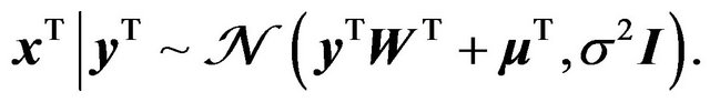 (3)
(3)
Then, the associated log-likelihood function is given by
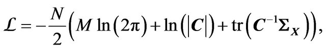 (4)
(4)
where  and
and  denote the determinant and the trace, respectively, of a matrix
 , and the sample covariance matrix is given by
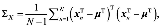 (5)
(5)
with  denoting the n-th observation (row of
 ). Notice also that the ML estimate for
  is given by the sample mean of the data. Finally, the estimates for the probabilistic principal components, that is, the columns of
  and the noise variance
 , are obtained by iterative maximization of Equation (4):
 (6)
(6)
 (7)
(7)
where the K columns of the  matrix
  are the principal eigenvectors of
 , with corresponding eigenvalues
 , constituting the
  diagonal matrix
 , and
, and  is an arbitrary
  orthogonal rotation matrix. In practice,
  is ignored by simply setting
 . Finally, the
  matrix
  whose columns are the probabilistic principal factors is simply obtained by projecting the data matrix on the probabilistic principal components, that is,
 (8)
(8)
2.3. Integration Measure via 2nd-Order Statistics
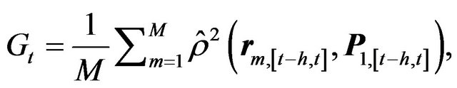
One of the main aspects of the proposed approach is the time-varying management of the risk, through an integration measure based on second-order statistics, which is applied on overlapping time-windows. More specifically, let h denote the window length and s the step size. Then, the integration measure we use at time t, Gt, is defined as
 (9)
(9)
where  is the squared correlation between two variables,
  denotes the first principal factor extracted by applying PPCA in the time window [t − h, t], and
  is the vector of returns of the m-th asset during the time interval [t − h, t]. The integration measure is computed by rolling the time window every s time steps, where the time-scale depends on our specific needs (e.g., daily, weekly, monthly).We interpret the periods when the returns are highly correlated to the first probabilistic principal component to be periods of high integration. We emphasize again that measuring and monitoring integration is crucial in the pure alpha framework, since a high integration period nominates decisions for decreased risk to be taken. Moreover, since our data have only equity indexes we can use this measure toassess integration assuming that most of the times equity markets are positively correlated.
2.4. Optimal Portfolio Strategies
2.4.1. Optimal Long-Short Portfolios
The construction of an optimal portfolio entails a meanvariance optimization over an ensemble of assets expected returns and a covariance matrix. For this purpose, accurate prediction of returns and covariances are required, with the former one, that is, the forecast of returns, being the most challenging part.
Concerning the estimationof the sample covariance matrix, an initial estimate is computed for each time window [t − h, t], which is then corrected using shrinkage (Stein’s estimator) [13,14] to improve the out-of-sample performance and reduce the estimation risk.
Market neutral portfolios are portfolios uncorrelated with the market, delivering positive returns. This is only possible through the use of short sales, the optimization program will return the long and short positions, with the additional property of being beta neutral. Among the advantages of market neutral investing, is its ability to enhance the performance of any index portfolio by combining an alpha strategy with an equity index. Our goal is to build a zero-beta portfolio by determining optimal long and short positions, under the constraint that portfolio’s beta should be equal to zero.
According to modern portfolio theory, an investor is interested in maximizing his utility , associated with a portfolio
 , with
  being an M-dimensional vector of weights (one weight per asset). The vector of optimal weights is obtained by solving the following optimization problem:
 (10)
(10)
 (11)
(11)
where  is the expected return of our portfolio, with
  being the vector of expected excess returns of the assets,
  is the portfolio’s variance, with
  being the estimated covariance matrix of the returns, and
  is the desired portfolio’s variance. In Equation (11),
  is a regularization parameter representing the investor’s level of risk aversion. In order to eliminate the exposure to the market or main factor, a beta constraint should be introduced:
where  is the M-dimensional vector of assets’ beta values calculated with an equally weighted index (EWI) as the market, and
  the portfolio’s beta. The constraint of zero portfolio’s beta yields an optimal portfolio which is not exposed to market risk. Motivated by [15], where it was shown that the principal orthogonal linear factor dominating the equity returns is highly correlated to an EWI, we justify the consistency of employing probabilistic principal factors to quantify co-movements among the distinct assets.
In addition, the EWI assumption results in the following simple expression for the vector of assets’ betas:
 (12)
(12)
where  is the M-dimensional vector of all ones.
We modify the approach introduced by [5] where earning yields are used to estimate the expected returns and a beta neutral portfolio is constructed, we suggest building a portfolio strategy based on a minimum variance portfolio, which does not require an estimate of expected returns. We have analyzed the properties of the betaneutral portfolio, which is a portfolio uncorrelated with the main factor explaining the returns of the set of assets in the system. We argue that this portfolio should be similar to a minimum variance portfolio. In fact, a beta neutral portfolio should neutralize the exposure to the principal factor or market factor, while a minimum variance portfolio will be the result of a mix of assets mainly related to the smallest risk factors. We can therefor build a minimum variance portfolio, which has been studied by other authors who argue that it is a more stable strategy than the full mean-variance optimization, in part because it does not rely on an estimate of expected returns.
In the case of a minimum variance portfolio, the objective function is modified such that only the risk part is optimized. The optimization problem in this case is then:
 (13)
(13)
As we mentioned above, we expected that the selected assets in the optimal minimal variance portfolios correspond to those highly related to the smallest factors and, in the same way, the market neutral portfolios will be composed of assets not highly related to the main factor, therefore related to factors of lower risk. The construction of portfolios with minimum variance is therefore an indirect way to build an alpha strategy.
2.4.2. Adjustment of Optimal Weights
Having calculated the optimal weights (long and short positions) by solving the optimization problem expressed by Equations (11) and (13), the second stage aims in adapting these weights so as to keep a constant risk through the strategy or to achieve a time-varying risk allocation. Two adjustmentsare considered: 1) reduction of the exposure to the market and enforcement to constant volatility of our portfolio for the initial strategy, and 2) adaptation of the corresponding weights by employing the values of the computed integration measure Gt for the scaled strategies.
As mentioned before, one the main purposes for monitoring the degree of integration through time is to warn investors for periods of high integration, where fewer opportunities are left to generate alpha, and thus, they should take more conservative decisions.
The approach introduced in [5] was the first attempt to account for time variations of a risk budgeting rule, which is of significant importance. This, in conjunction with the robustness of the extracted probabilistic principal factors against potentially distinct noise levels across time or among different assets, as well as the inherent property to account for corrupted values in the original data, make our proposed portfolio construction method even more powerful when compared with the method introduced in [5].
More specifically, the integration measure Gt, given by Equation (9), is employed to decide for the units of risk, which could be taken at each period of time.The rule we propose for the adaptation of the weights  is as follows: for small integration values, the portfolio is allowed to have the maximum risk exposure, which is equivalent to using the optimal weights obtained from the solution of the optimization problem defined by Equation (11). On the other hand, for high integration values, the risk is reduced by reducing the weights of every position proportionally to its integration value.
The vector of optimal weights  is scaled by an appropriate scaling factor resulting in the following scaled weights
 (14)
(14)
where  is the integration value at time t after removing the mean computed over all the overlapping windows, so as to use the same thresholds for the whole time period of study. The lower and upper bounds of the integration,
  and
and , respectively, are thresholds which specify when the integration is low, and therefore higher possibilities to generate alpha exist, and when the integration reaches an upper limit, above which there are very few chances to generate alpha. Equation (14) implies that the optimal weights
  are modified linearly for integration values ranging in the interval
 , while for integration values larger than
  the weights are set equal to zero and for integration values smaller than
  the optimal weights are left unchanged. In practice, the values of the two thresholds
  and
and  can be set based on the quantiles of the distribution of the historical integration measure.
3. Experimental Evaluation
The proposed PPCA-based approach to analyze a dataset is used to measure integration and build alpha generating portfolio strategies for a set of financial data. We analyzed a group of 12 developed equity markets (Australia, Canada, France, Germany, Hong Kong, Japan, Singapore, Spain, Sweden, Switzerland, United Kingdom, and USA), for which liquid index futures contracts are available in order to enable short positions in the portfolio strategies.
Closing prices at a daily frequency for the main futures indexes of each country have been collected, expressed in local currency, covering the period between January 2001 and January 2013. The use of data in local currencies can be advantageous in terms of diversification of international portfolios, however any undesired exposure to a specific currency can be hedge using several methods which do not need to be considered in this study.
During the selected time period, all markets had undergone through the two main markets crisis of recent years: the IT-bubble and the subprimes and debt crisis. Both crises are followed by a recovery period, thus, offering a good opportunity to study integration and longterm portfolio strategies. We note also that, in order to emphasize the short-run movements of the data, the relative change between consecutive time instants is used. This can be measured by computing the first difference of the natural logarithm (dlog) of the time-series samples. Thus, a preprocessing step is applied on the original ensemble of the M time-series as follows:
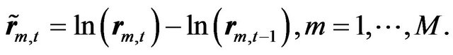 (15)
(15)
Besides, to overcome the limitation of significantly different variances or expression in different units (as it is the case in our dataset with the different currencies) between the several time-series, a further normalization to zero mean and unit variance of the dlog time-series is performed. The performance of the proposed method is evaluated for a window length h = 250 and step-size s = 25.
3.1. Performance Measures
To analyze the risk-adjusted performance of the different portfolio strategies we use three different indicators [16]: 1) the Sharpe ratio (SR), 2) the Sortino ratio (SoR) and 3) the maximum drawdown (MDD). For all these three measures we define  as the portfolio’s return and
  as the return of a risk free asset.
The Sharpe ratio is defined as the ratio of the average excess return of an asset over the risk-free rate and the volatility of this excess return:
 (16)
(16)
This ratio is the most common risk-adjusted performance measure used in financial studies. Its main drawback is that it is only useful for symmetrical distributions of returns.
The Sortino ratio is a variation of the Sharpe ratio, where the return is adjusted by the downside volatility, the volatility calculated only with negative returns. The Sortino ratio is defined as
 (17)
(17)
Since it takes into account the skewness of the distribution of returns, it would therefore be a better risk-adjusted performance indicator for payoffs with higher downside risk.
The maximum drawdown, which is defined as the maximum cumulated continuous loss over a given period, measures the degree of extreme losses. We also present the ratio of the maximum drawdown divided by the volatility, which indicates the degree of extreme loss in terms of the standard deviation of the returns. In particular, a lower maximum drawdown could be associated with lower overall risk. Moreover, this ratio standardizes the MDD measure in order to make it possible to compare payoffs with different volatilities.
3.2. Extraction of Probabilistic Principal Factors
In this section, the characteristics of the probabilistic principal factors extracted with PPCA are exhibited for the complete dataset. Figure 1 shows the correlation coefficients for the 12 market indexes from the initial data set. As it can be seen, all markets are positively correlated, with the highest correlation appearing between the CF1 and GX1 indexes compared to Z1 and ES1 indexes.
For a visual inspection of the difference between the principal components extracted with PCA and PPCA, Figure 2 shows the loadings of the original data  in the space of the first two principal components, for the whole time period. We observe that the effect of the probabilistic approach for the specific dataset results in a scaling and rotation of the principal axes, when compared with the typical PCA. Concerning the discriminative capability of both PCA and PPCA, at least for the first two principal components, the same behavior is observed, that is, the second principal components can be used to split the original variables (indexes) into the same two subsets.
However, one of the major advantages of PPCA, in contrast to PCA, is its ability to estimate simultaneously the underlying noise variance . This feature can be very important for further processing, such as, for designing adaptive and more accurate predictors of the local or global trends, by taking into account the spurious variations caused by the underlying noise. In Figure 3, the time-varying estimated noise variance is shown for (h, s) = (250, 25). As it can be seen, large variations of the estimated noise variance appear across time, thus, reveal-
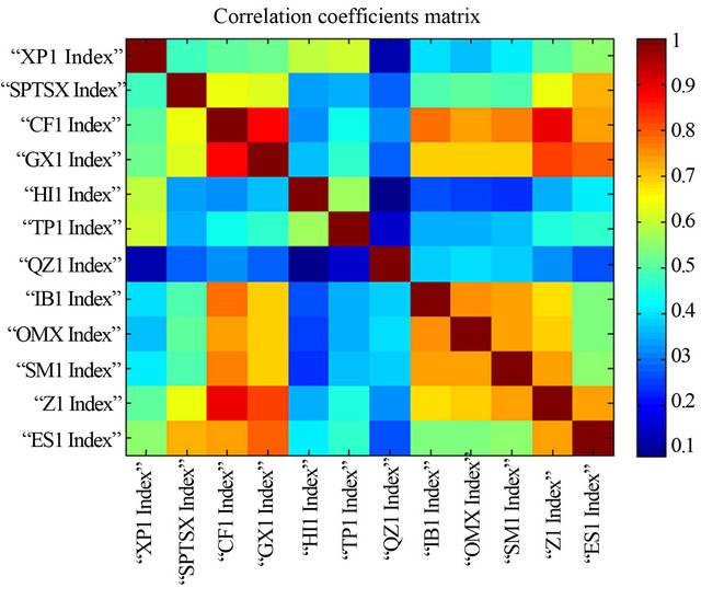
Figure 1. Correlation coefficient matrix of the 12 indexes.
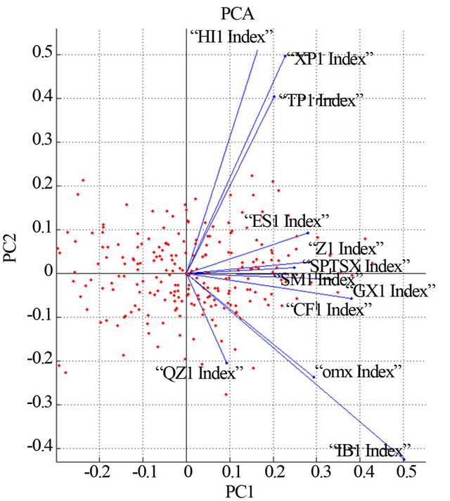
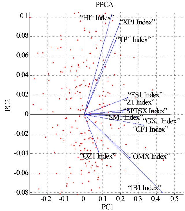
Figure 2. PCs for each variable (index) and PC score for each observation.
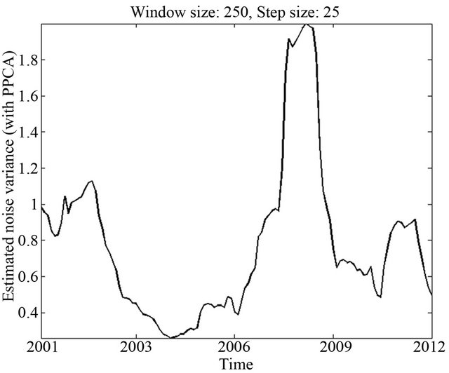
Figure 3. Estimated noise variance for (h, s) = (250, 25).
ing the significance of its accurate estimation for further actions, such as, trend estimation and forecasting. Moreover, interestingly, the noise variance acquires its local maximum values in periods close to the periods of crises.
Concerning the evolution of the integration measure Gt, Figure 4 shows the values of Gt for the PCA and PPCA, for (h, s) = (250, 25). As it can be seen, the dominant principal component extracted by both PCA and PPCA results in the same mean squared correlations with the 12 market indexes. This was expected, since from Figure 2, PPCA results in scaled and slightly rotated principal components.
Although the integration measure defined by Equation (9) results in similar values for both PCA and PPCA, we emphasize once again the superiority of our PPCA-based approach, which is also capable of monitoring the timevarying behavior of the underlying noise component, as well as its robustness against corrupted data, as it will be shown experimentally in a subsequent section.
3.3. Long-Short Strategies Payoffs
In this section, the efficiency of the proposed optimal portfolio construction method is evaluated. More specifically, the portfolio positions are calculated as the minimum variance optimal weights. Besides, the risk is controlled after each optimization by adjustment of the weights to a target volatility of 10%. As our optimized portfolio has long and short positions, it is possible to decrease (increase) the overall portfolio risk by reducing (enlarging) each position by a given proportion.
In the optimization process, the matrix  is used, which is obtained from a historical covariance matrix adjusted with a shrinkage method. We build a minimum variance portfolio at each estimation date with the shrunk covariance matrix estimated from the matrix of excess returns for each window. The proposed strategy has a Sharpe ratio of 0.20%, a Sortino ratio of 0.35%, and a maximum drawdown of 44.3%. The results are summarized in Table 1.
Integration is calculated for rolling windows of one
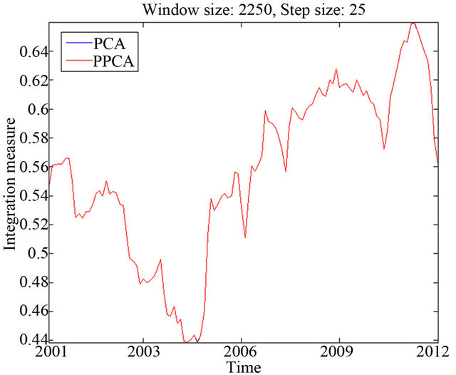
Figure 4. Integration measure Gt for PCA and PPCA, with (h, s) = (250, 25).
year length (h = 250) every 25 observations. As we mentioned before, we have observed that high integration allows very few opportunities to generate alpha. This is illustrated in Figure 5, which shows the time-relation between our proxy of market integration and the minimum variance strategy.
We observe that the strategy suffers during periods of high integration of the equity markets. In addition, integration spikes during periods of crisis, which make this information useful to adjust the total risk taken at each date.
We construct a scaling factor for our long-short weightsbased on the level of integration in order to structure a downside protection that alerts during periods of high integration, when the market is highly drifted and there are few possibilities of alpha generation. The idea is to transform the integration measure, which is a variable defined in the range [0,1], where 1 indicates perfect integration and 0 indicates no integration, into a variable defined in the same range but where 1 indicates that the optimal weights from the optimization should be considered and 0 indicates that no risk should be taken.
Three simple scaling methods are employed to transform the integration level: 1) , 2) using Equation (14), for levels of Gt between
  and
and  and outside their
Table 1. Risk adjusted performance measures.
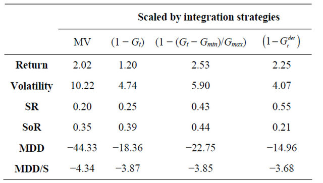
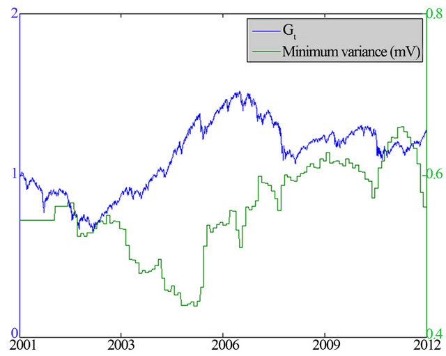
Figure 5. Minimum variance strategy and integration.
range we set the levels equal to 0 for  and equal to 1 for
  and 3)
 ,where
  is the linearly de-trended series of
 . The optimal weights are scaled according to these three methods and the performance of each strategy is computed. For the second scaling method, we set the parameters
  to be the 20th percenttile of
  observed up to the estimation point and
  to be equal to the 80th percentile that we consider a high level of integration.
The average value of  for the whole period of study is 0.56. The minimum
  for the whole series of observations is 0.43 and
  is 0.66. We compare the basic minimum variance strategy with the different proposed strategies with the risk adjusted by integration. Sharpe ratios improve from 0.2 to 0.41 on average for the scaled strategies. The Sortino ratio is equal to 0.35 for the basic strategy and does not change on average for the risk budgeting strategies. However, it is different for each of the three scaling methods. The ratio of maximum drawdown over volatility varies from 4.34 to 3.80, resulting in a 0.54 improvement of standard deviation.
The best of the three scaling methods is shown to be the third one, which improves the Sharpe ratio of the standard minimum variance strategy from 0.20 to 0.55 and the ratio of maximum drawdown over volatility from 4.34 to 3.68, while the size of the extreme loss of the strategy is reduced by 0.66 standard deviations. All the above results are summarized in Table 1.
It is also important to note that all the scaled strategies have improved the risk-adjusted performance indicators. As a general conclusion we see that the use of a time-varying risk budgeting, based on an integration measure expressed in terms of the dominant probabilistic principal factor, improves the payoff of the basic minimum variance strategy with the protection against loses during certain critical periods.
Figure 6 presents the basic minimum variance portfolio strategy compared to the improved by integration scaling strategies. We observe that the risk-budgeting strategies are characterized by reduced levels of risk during the periods of high integration, which was exactly our desired goal.
3.4. Performance of PPCA with Missing Data
In this section, we study the robustness and efficiency of PPCA to extract the dominant principal factors, and subsequently to calculate the integration measure  in case of missing data. This is often the case when we don’t have full access to some closing values of the market indexes, or when those values may be hidden on purpose. We emphasize that, in contrast to previous approaches, it is not required to fill in the missing data, but PPCA proceeds by fitting the remaining data with a probabilistic model. This capability is not available with the standard PCA, which would need the reconstruction of the missing observations in some way, prior to the construction of the optimal portfolio. We also note that the advantage of PPCA to extract accurately the principal factors to be used for the calculation of the associated integration measure in case of missing data cannot be incorporated in the current portfolio optimization strategy. The reason is that, apart from the integration measure, the proposed risk-budgeting strategies also employ the full data prior to the current date, which requires filling in the missing data. However, the design of appropriate strategies without necessitating the recovery of missing values is left as a separate study.
In order to evaluate the efficiency of PPCA to extract principal factors and estimate accurately the underlying noise variance in case of missing data, a varying percentage  of missing elements from the original log-returns matrix
  is ignored uniformly at random.
Figure 7 shows first that the PPCA-based approach is robust in estimating accurately the variance of the underlying noise component, even in the extreme scenario of 50% of missing values. Finally, and most importantly, Figure 8 verifies the efficiency of the proposed simple integration measure between the given market indexes and the dominant probabilistic principal factor, even for an extreme situation of missing observations at the order of 40% of the original data.
4. Conclusions and Future Work
In this paper, we introduced a portfolio optimization method for pure alpha investments, by exploiting a market integration measure based on second-order statistics between the original data and the dominant probabilistic principal factor. The proposed time-varying risk-budgeting strategies were characterized by reduced levels of risk during the periods of high integration, thus, verifying the efficiency of our method to be used as an alerting

Figure 6. Minimum variance strategy compared to scaled strategies with the integration measure Gt based on PPCA.
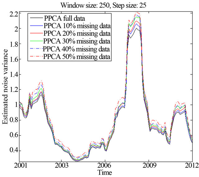
Figure 7. Estimated noise variance for (h, s) = (250, 25), and for a varying percentage of missing observations  .
.
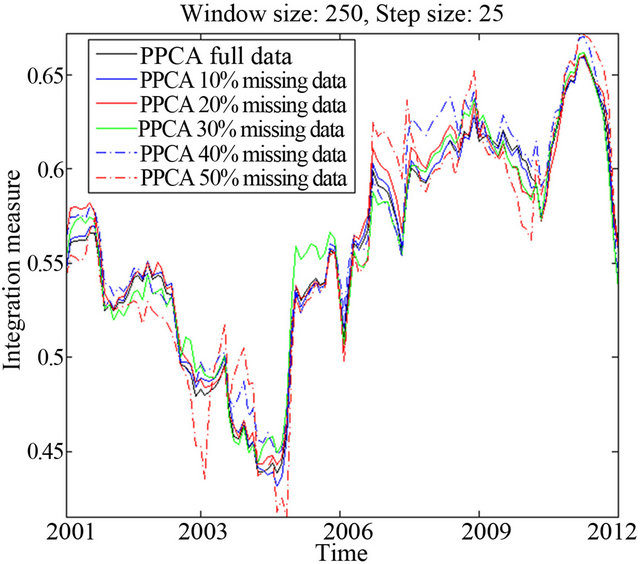
Figure 8. Integration measure Gt for PPCA, with (h, s) = (250, 25), and for a varying percentage of missing observations .
.
mechanism for pure alpha investors.
As a future work, the time-varying estimated noise variance, which is a byproduct of the method presented in this study, will be further exploited to design efficient algorithms for estimating and predicting local and global trends, by taking into account the spurious variations caused by the underlying noise component. Moreover, due to the market-neutral property, which is inherent in our method, the proposed alpha strategy will be combined with an index portfolio (or any other portfolio strategy) to achieve an overall increase of the portfolio optimization performance.
REFERENCES
- R. Merton, “Lifetime Portfolio Selection under Uncertainty: The Continuous Time Case,” Review of Economics and Statistics, Vol. 51, No. 3, 1969, pp. 247-257. doi:10.2307/1926560
- J. Campbell and L. Viceira, “Consumption and Portfolio Decisions when Expected Returns Are Time Varying,” Quarterly Journal of Economics, Vol. 114, No. 2, 1999, pp. 433-495. doi:10.1162/003355399556043
- R. Bansal, M. Dahlquist and C. Harvey, “Dynamic Trading Strategies and Portfolio Choice,” NBER Working Paper, 2004.
- M. Brandt and P. Santa-Clara, “Dynamic Portfolio Selection by Augmenting the Asset Space,” Journal of Finance, Vol. 61, No. 5, 2006, pp. 2187-2217. doi:10.1111/j.1540-6261.2006.01055.x
- J. Caicedo-Llano and T. Dionysopoulos, “Market Integration: A Risk-Budgeting Guide for Pure Alpha Investors,” Journal of Multinational Financial Management, Vol. 18, No. 4, 2008, pp. 313-327. doi:10.1016/j.mulfin.2008.01.002
- W. Sharpe, “Capital Asset Prices: A Theory of Market Equilibrium under Conditions of Risk,” Journal of Finance, Vol. 19, No. 3, 1964, pp. 425-442.
- M. Tipping and C. Bishop, “Probabilistic Principal Component Analysis,” Journal of the Royal Statistical Society, Series B, Vol. 61, Pt. 3, 2002, pp. 611-622.
- M. Gordon, “The Investment, Financing, and Valuation of the Corporation,” American Economic Review, Vol. 52 No. 5, 1962.
- J. Campbell and Y. Hamao, “Predictable Stock Returns in the United States and Japan: A Study of Long-Term Capital Market Integration,” Journal of Finance, Vol. 47, No. 1, 1992, pp. 43-69. doi:10.1111/j.1540-6261.1992.tb03978.x
- G. Bekaert and C. Harvey, “Time Varying World Market Integration,” Journal of Finance, Vol. 50, No. 2, 1995, pp. 403-444. doi:10.1111/j.1540-6261.1995.tb04790.x
- M. Fratzscher, “Financial Market Integration in Europe: On the Effects of EMU on Stock Markets,” ECB, Vol. 48, 2001.
- J. Caicedo-Llano and C. Bruneau, “Co-movements of International Equity Markets: A Large-Scale Factor Model Approach,” Economics Bulletin, Vol. 29, No. 2, 2009, pp. 1466-1482.
- P. Jorion, “International Portfolio Diversification with Estimation Risk,” Journal of Business, Vol. 58, No. 3, 1985, pp. 259-278. doi:10.1086/296296
- M. Daniels and R. Kass, “Shrinkage Estimators for Covariance Matrices,” Biometrics, Vol. 57, No. 4, 2001, pp. 1173-1182. doi:10.1111/j.0006-341X.2001.01173.x
- S. Heston, K. Rouwenhorst and R. Wessels, “The Structure of International Stock Returns and the Integration of Capital Markets,” Journal of Empirical Finance, Vol. 2, No. 3, 1995, pp. 173-197. doi:10.1016/0927-5398(95)00002-C
- J. Campbell and R. Shiller, “Valuation Ratios and the Long-Run Stock Market Outlook: An Update,” Cowles Foundation Discussion Papers, 2001.