Journal of Mathematical Finance
Vol.3 No.1(2013), Article ID:28162,11 pages DOI:10.4236/jmf.2013.31005
Stochastic Control for Asset Management
1Department of International Business, Ming Chuan University, Taipei, Taiwan
2Department of Economics, Hong Kong Baptist University, Hong Kong, China
3Department of Finance, Providence University, Taichung, Taiwan
Email: fnjames@mail.mcu.edu.tw, awong@hkbu.edu.hk, wuec@pu.edu.tw
Received May 6, 2012; revised August 7, 2012; accepted August 19, 2012
Keywords: Stochastic Control; Three-Asset Model; Vasicek Interest Rate Model; Optimal Fraction
ABSTRACT
An investor is often faced with the investment situation in which he/she has to decide how to allocate his/her limited funds optimally among different assets to maximize his/her expected utility over the holding period. To this end, this study sets up a dynamic model driven by three assets to characterize the stochastic nature of the securities market and uses stochastic control to derive an explicit formula for the optimal fraction invested in each of the three assets for an investor with a power utility and a holding period of 10 years. Using estimated parameter values as inputs and implicit finite difference method, we determine numerically the optimal percentages invested in the three assets at each time over the holding period for both less risk-averse and more risk-averse investors.
1. Introduction
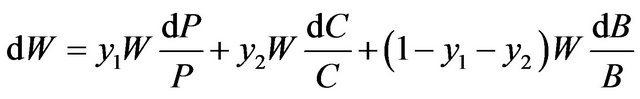
Modern portfolio theory1 is generally regarded to have started with the mean-variance (M-V) analysis of Harry M. Markowitz [1]. Using the means and variances (or equivalently expected returns and standard deviations) of asset returns as the criteria for portfolio management, Markowitz showed how to create a frontier of investment portfolios over a single holding period [0,T] such that each of them has the greatest possible expected return, given their level of standard deviation or risk. Under the M-V assumptions, we obtain the two-fund separation theorem2 [4,5] which states that an investor, based on his degree of risk averseness, decides at initial time 0 to hold a certain combination of the risk-free asset and the market portfolio3 so as to maximize his expected utility at terminal time T. For example, at time 0, a conservative investor will allocate a smaller percentage of his funds to the market portfolio whereas an aggressive investor will allocate a larger percentage to the market portfolio. Once the allocation of funds has been made at time 0 between the two assets, M-V analysis dictates that no further trading will be done by the investor until time T.
M-V analysis presupposes that the rate of return on the risk-free asset and the expected returns and standard deviations of risky assets do not change over the holding period. It is not too incorrect to assume that they remain unchanged for short holding period (e.g., three or six months), but it is inaccurate to assume that they remain unchanged for long holding period (e.g., five years or longer). For long period, an M-V model under such presupposition is obviously an unreasonable approximation to the actual securities market. In fact, numerous empirical studies have attested the dynamic and stochastic nature of interest rates [10-12] and asset prices [13-19]. For example, many studies [13,15,17,18] have found marked negative long-term serial correlation in stock returns, which may result from a combination of a changing expected return and expected return reverting to its mean over time. Hence, asset management based on static M-V models is bound to err for long holding period.
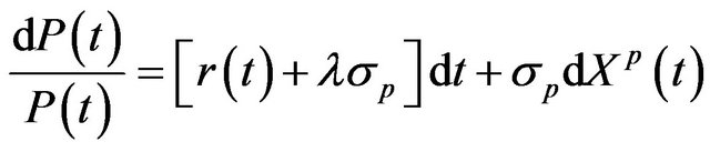
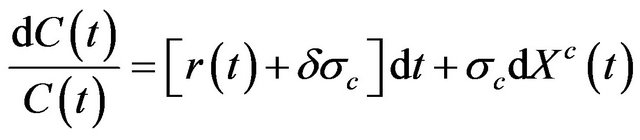
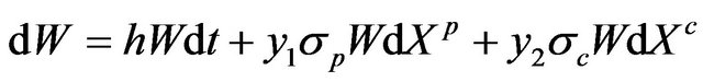
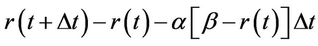
In this study, we employ stochastic differential equations to characterize the dynamic and stochastic nature of the prices of the underlying assets in a securities market. In addition, we use stochastic control to derive a formula for the optimal fraction (i.e., optimal control) invested in each of the assets at each time over the holding period. To adequately depict the stochastic nature of the securities market, we assume that it is driven by the following three assets4: a risk-free asset (a short bond), a risky asset (a market index), and another risky asset (a long bond). For the risk-free asset, we assume that its underlying risk-free rate or short rate follows the Vasicek [24] interest rate model. The reason for using the Vasicek model is its mean-reverting property. Under the Vasicek model, the short rate will tend to be pulled back to some longrun average level over time when it is either too high or too low. For each of the two risky assets, we assume that the drift of its price is made up of the short rate plus an appropriate risk premium (we will estimate the two risk premiums in Section 3) whose magnitude depends on the riskiness of the asset. Such characterization of the prices of the two risky assets is consistent with many empirical findings [13,15,17,18] for asset prices.
To sum up, in M-V models, an investor, based on his degree of risk averseness, can decide ONLY at initial time 0 how to divide his funds between the risk-free asset and the market portfolio (often an index fund in practice) to maximize his expected utility at time T. In our threeasset model, an investor, based on his degree of risk averseness, can determine at EACH time over the holding period the optimal allocation between the three assets (i.e., short bond, long bond, and market index) to maximize his expected utility at terminal time T. As such, our model is superior to M-V models in that ours is dynamic but theirs is static.
The rest of the paper proceeds as follows. In Section 2, we set up a dynamic model driven by three assets and use stochastic control to derive an explicit formula for the optimal fraction of wealth invested in each of the three assets. In Section 3, we use maximum likelihood method to estimate the relevant parameters of our model. Section 4 shows how to implement our model numerically using implicit finite difference method. In Section 5, we report the optimal percentage invested in each of the three assets at times t = 2 and 8 over a holding period of ten years for two types of investors (one type is less riskaverse and the other more risk-averse). Section 6 concludes this study.
2. Optimal Fraction for a Three-Asset Model
Our three-asset model involves a risk-free asset, a risky asset, and another risky asset. Let  be the price of the risk-free asset,
  be the price of the first risky asset, and
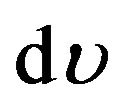
  be the price of the second risky asset. We assume that the instantaneous rate of the risk-free asset is the short rate
 , the expected rate of return on the first risky asset is
 , and the expected rate of return on the second risky asset is
 . Hence, we have
 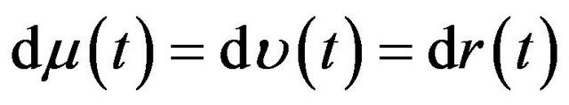 . Accordingly, we describe the dynamics of the short rate and the three asset prices by the following stochastic differential equations:
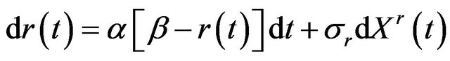 , (1)
, (1)
 , (2)
, (2)
 , (3)
, (3)
 , (4)
, (4)
where ,
,  , and
, and  are standard Brownian motions with
 ,
,  , and
, and . In the following, we form a three-asset portfolio such that we invest a fraction
  of our wealth
  in the first risky asset,
  in the second risky asset, and the rest
  in the riskfree asset. Then, the dynamics of wealth
  can be written as
 . (5)
. (5)
Substituting ,
,  , and
, and  of (2), (3), and (4)
into (5) and simplifying the equation, we have
 (6)
(6)
where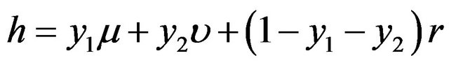 . Letting
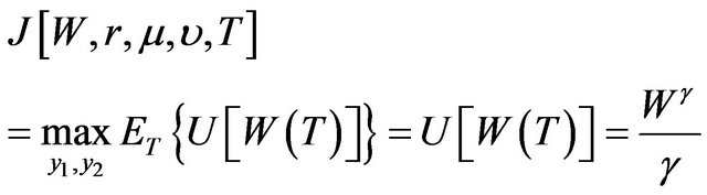
 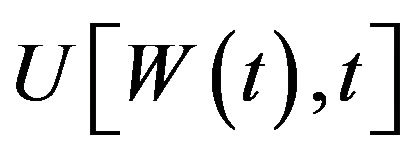 be a strictly concave-shaped utility [4,25] defined over wealth and assuming that the investor allocates his wealth between the three assets so as to maximize his expected utility at terminal time T, we obtain the maximized utility function
 at time
  such that
 (7)
(7)
subject to the budget constraint of (6). The fact that the utility function is strictly concave implies that the investor is risk averse. In this study, we assume power utility
 (where
  is the risk averseness parameter) for the investor. There are two reasons for using power utility. One is that an explicit solution can be obtained for our model with power utility [26-29], but not with other utility functions (e.g., exponential or quadratic utility). The other is that power utility leads to an optimal solution which is independent of wealth and thus will greatly simplify the derivation. In fact, empirical evidence [4,25] suggests that the typical utility of an investor is characterized by decreasing absolute risk averseness and constant relative risk averseness. These properties are consistent with power utility.
With no money added or withdrawn from our threeasset portfolio at any time , the maximized utility function
  at time
  is
is
 . (8)
. (8)
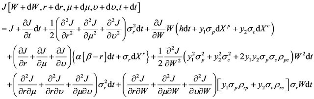
Letting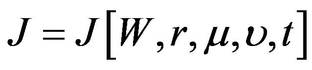 and expanding
by applying Taylor’s theorem, we obtain
 (9)
(9)
where ,
,  ,
,  ,
,
 , and
, and .
.
Substituting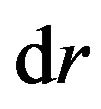 ,
,  ,
,  ,
,  ,
,  ,
,  ,
,  ,
,  ,
,  ,
,  ,
,  ,
,  ,
,  , and
, and  into (9), we get
 (10)
(10)
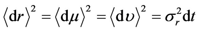
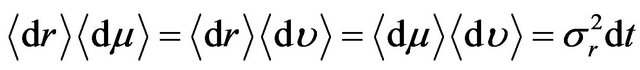
Taking expectation of (10) and noting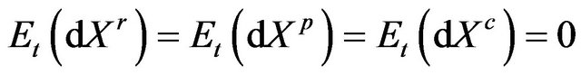 , we have
 (11)
(11)
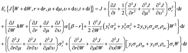
Substituting (11) into (8) and dividing each side by dt, we obtain the following Hamilton-Jacobi-Bellman (HJB) equation:
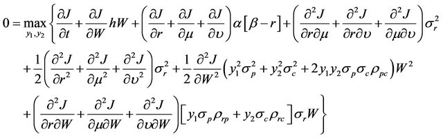 (12)
(12)
To solve the HJB equation, we first let
 , where
  is any positive function. With no consumption until time T, we have
 .
.
Thus, we have . For simplicity, we let
 . Given
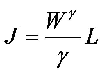 , we have
 ,
,  ,
, 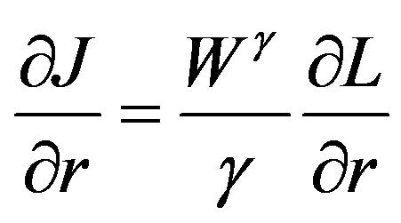 ,
,
 ,
,  ,
, ,
,
 ,
,  ,
,  ,
,
 ,
,  ,
,
 ,
,  ,
,
 ,
, .
.
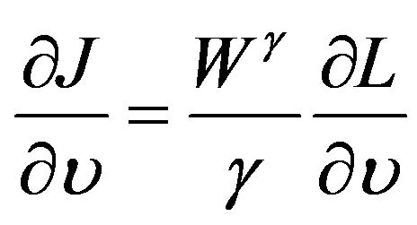
After replacing J-related terms by L-related terms in (12) and simplifying the equation, we obtain
 (13)
(13)
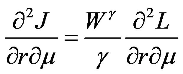
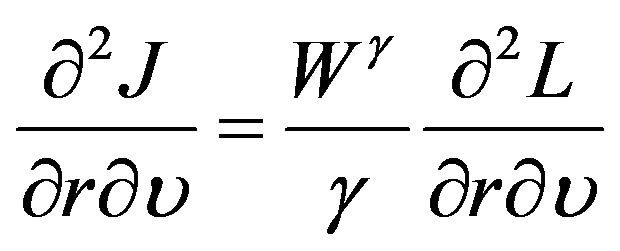
where . Collecting terms involving
  and
and  in (13) and rearranging, we obtain
 (14)
(14)
where
 .
.
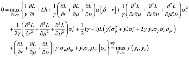
We note that  does not involve
  and
and . Furthermore, by setting
 , we obtain the first-order conditions to maximize equation in (14) such that
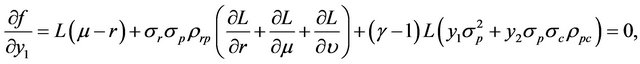 (15)
(15)
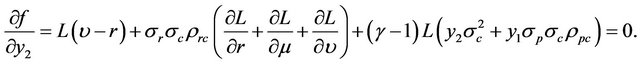 (16)
(16)
Solving (15) and (16) for  and
and , we obtain the following optimal fractions
 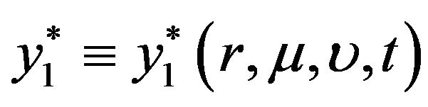 and
and 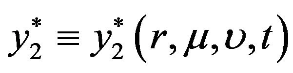 invested in the first and second risky assets, respectively, at time
 :
:
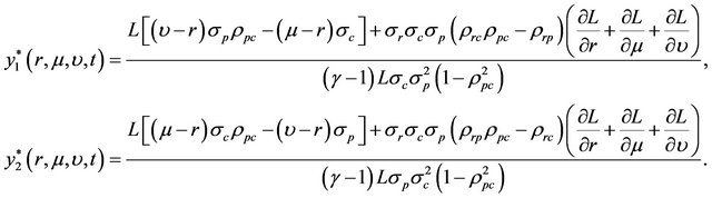 (17)
(17)
Correspondingly, the optimal fraction invested in the risk-free asset is .
.
3. Empirical Estimation of the Parameters
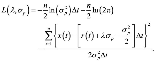
As mentioned in Section 1, the securities market is assumed to be driven by the following three assets: a risk-free asset (a short bond), a risky asset (a market index), and another risky asset (a long bond). In this section, we estimate the parameters in (1), (3), and (4) by using the maximum likelihood (ML) method [30]. ML estimation is based on large sample asymptotic estimators, which are asymptotically normally distributed. Since we use 30 years of daily price data for estimation, the ML estimates so obtained should be accurate.
Three sets of data, a total of 7826 daily price observations from 2 January 1978 to 31 December 2007, are used for estimation. One set is the 3-month US Treasury bill rate (retrieved online from the database of the US Federal Reserve Bank of St. Louis) and the other two sets are the S&P 500 Index value and the 10-year US government bond price (both retrieved from the Datastream database). We use the 3-month Treasury bill rate to proxy for the short rate , the S&P 500 Index5 for the price
  of the first risky asset, and the 10-year US government bond for the price
  of the second risky asset.
The stochastic differential equation (SDE) in (1) can be expressed in discrete form as follows:
 (18)
(18)
where  is a standard normal deviate and
 is distributed as
 . With a sample size of n, the natural logarithm of the likelihood function
 , considered as a function of
 ,
,  , and
, and , can be written as
 (19)
(19)
The SDE in (3) can be expressed in discrete form as follows:
 (20)
(20)
where  is a standard normal deviate. Given that
 and
and , the logarithm of price relatives
  is normally distributed with mean
  and variance =
 . With a random sample size of n, the natural logarithm of the likelihood function
 , considered as a function of
  and
and , can be written as
 (21)
(21)
The SDE in (4) can be expressed in discrete form as follows:
 (22)
(22)
where  is a standard normal deviate. Given that
 and
and , the logarithm of price relatives
  is normally distributed with mean =
 and variance =
 . With a random sample size of n, the natural logarithm of the likelihood function
 , considered as a function of
  and
and , can be written as
 (23)
(23)
ML estimates are found by maximizing (19) with respect to ,
,  , and
, and  using the 3-month Treasury bill rates, by maximizing (21) with respect to
  and
and  using the S&P 500 Index value, and by maximizing (23) with respect to
  and
and  using the 10-year US government bond prices. The estimates for the seven parameters are as follows:
 ,
,  ,
,  ,
, 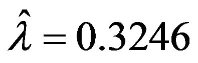 ,
, 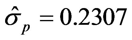 ,
, 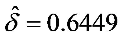 , and
, and .
.
4. Implementation by Implicit Finite Difference Method
In this study, we use a 10-year holding period. For implementation, we first transform the domain of our continuous problem into a discretized domain. Hence, we partition our 10-year holding period [0,T] into m equal intervals of length 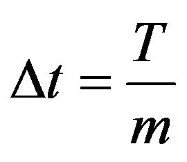 such that there are
trading times indexed by . At each time
  (where
 ), we construct a three-dimensional grid with three axes representing
 ,
,  , and
, and , where
  ranges from 0.01 to 0.12,
  from 0.03 to 0.20, and
  from 0.03 to 0.015. That is, point
  on the grid at time
  corresponds to
 ,
,  , and
, and  , where
 ,
,  , and
, and . With the above setup, we determine numerically the optimal percentages invested in each of the three assets at each point on the three-dimensional grid at each time based on (17).
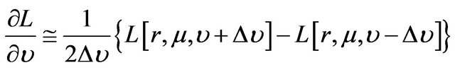
To implement, we use implicit finite difference method to compute numerically the partial derivatives of . Specifically, the partial derivatives are first converted into a set of difference equations and these difference equations are then computed iteratively backward in time. Accordingly, the firstand second-order partial derivatives of
  are approximated by the following finite difference operators [31-33] in which, for simplicity, we suppress the argument t of
 :
:
 , (24)
 , (25)
 , (26)
 , (27)
 , (28)
 , (29)
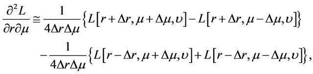 (30)
(30)
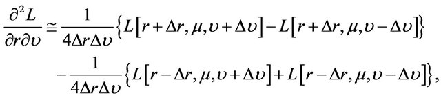 (31)
(31)
 (32)
(32)
The algorithm begins at time 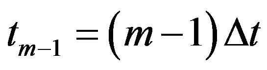 and works backward in time. For each point on the threedimensional grid at time
 , we compute the value of
  from the value of
 , where
  at time T for all values of
 ,
,  , and
, and . The values of
  and
and
 are computed from the values of
  using (17). At time
 , we compute the value of
  from the value of
  and then the values of
  and
and  are computed from the values of
 . This algorithm is done iteratively until we reach time
 . To ensure satisfactory convergence, we use a small value of 0.001 for
 . Hence, for a 10-year holding period, the number of intervals is
 .
.
5. Numerical Results
As pointed out in Section 2, we assume that the investor has a power utility , where
  is the risk averseness parameter. Note that an investor with a larger
  means that he is more risk averse. Copeland et al. [4] used a power utility with
  and Brennan et al. [34] used a power utility with
 . Hence, we set
  for less risk-averse investors and
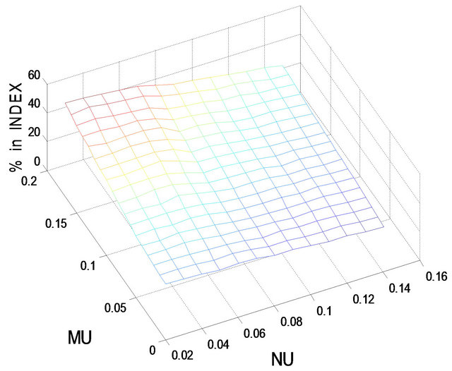
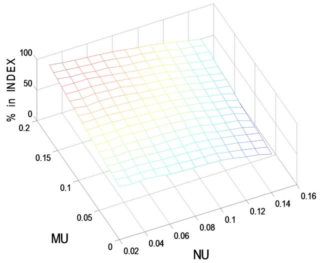
  for more risk-averse investors. In the following, we use Figures 1-4 to show the optimal percentages for the former in Subsection 5.1 and Figures 5-8 to show those for the latter in Subsection 5.2. In each figure, fixing r = 0.02 and then r = 0.08, we examine how their optimal percentages in market index (panel A) and long bond (panel B) change for different
  and
and .
.
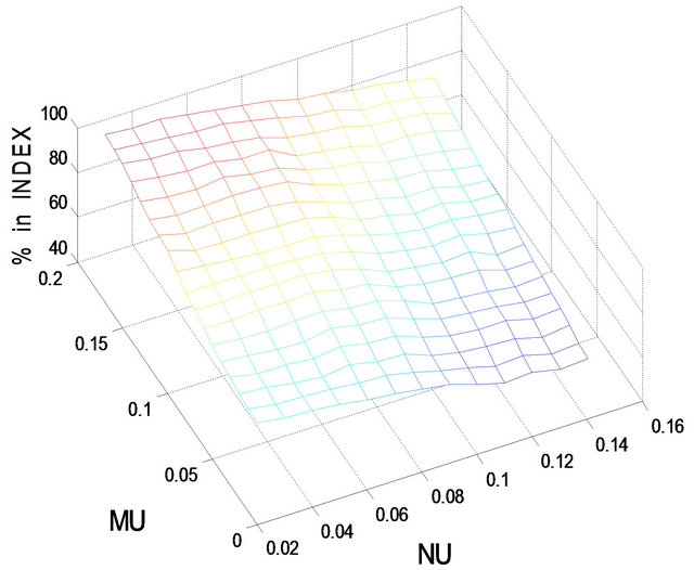
In Figures 1-8, note that (1) we use MU for  and NU for
  and (2)
  = optimal percentage in short bond, where
  = optimal percentage in market index and
  = optimal percentage in long bond. For example, in Figure 1,
 (a)
(a)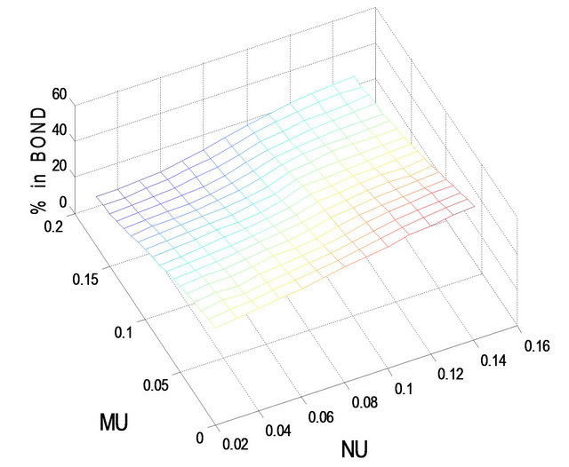 (b)
(b)
Figure 1. Optimal percentages in index and long bond at  and
and  when
when .
.
 (a)
(a) (b)
(b)
Figure 2. Optimal percentages in index and long bond at  and
and  when
when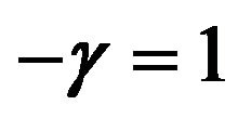 .
.
 (a)
(a)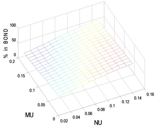 (b)
(b)
Figure 3. Optimal percentages in index and long bond at  and
and  when
when .
.
 (a)
(a)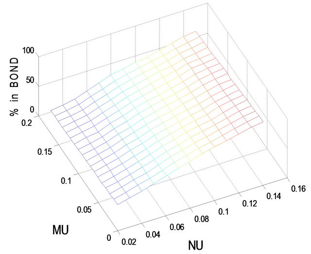 (b)
(b)
Figure 4. Optimal percentages in index and long bond at  and
and 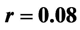 when
when .
.
 (a)
(a) (b)
(b)
Figure 5. Optimal percentages in index and long bond at  and
and  when
when .
.
 (a)
(a)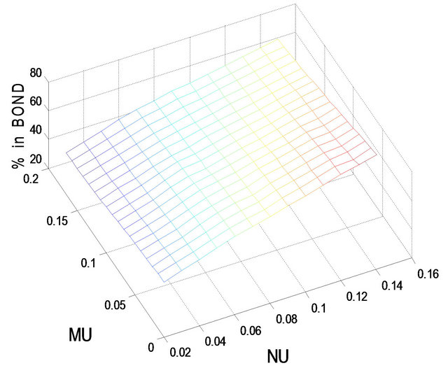 (b)
(b)
Figure 6. Optimal percentages in index and long bond at 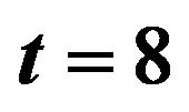 and
and  when
when .
.
 (a)
(a)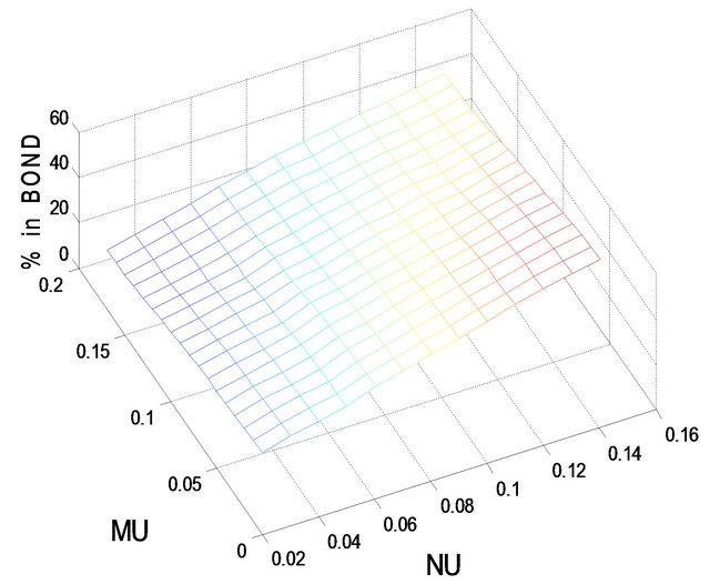 (b)
(b)
Figure 7. Optimal percentages in index and long bond at  and
and  when
when .
.
 (a)
(a)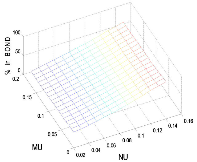 (b)
(b)
Figure 8. Optimal percentages in index and long bond at  and
and  when
when .
.
 and
and  when
when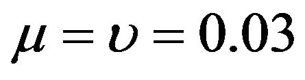 . Hence the optimal percentage in short bond =
  , given t = 2, r = 0.02, and
 .
.
5.1. Optimal Percentages for Less Risk-Averse Investors
Figures 1 and 2 show the optimal percentages in market index and long bond at, respectively, t = 2 and 8 when r = 0.02. In Figures 1 and 2, the optimal percentage ( ) in market index increases as
  increases and decreases as
  increases. For example, in Panel A of Figure 1, given
 ,
,  increases from 61.3% when
  to 91.8% when
 ; on the other hand, given
 ,
,  decreases from 64.9% when
  to 48.8% when
 . In Figures 1 and 2, the optimal percentage (
 ) in long bond decreases as
  increases and increases as
  increases. For example, in panel B of Figure 2, given
 ,
,  decreases from 77.4% when
  to 58.2% when
 ; on the other hand, given
 ,
,  increases from 56.4% when
  to 79.1% when
 . The value of
  has a notable effect on the optimal percentages. Specifically, other things held fixed (r = 0.02 for one thing), the optimal percentage in market index decreases but that in long bond increases as t increases from 2 to 8. For example, given
 ,
,  decreases from 63.2% when t = 2 to 19.2% when t = 8, whereas
  increases from 36.2% when t = 2 to 70.2% when t = 8. Apparently, there is a substitution effect at work between market index and long bond as the holding period becomes shorter. In addition, given r = 0.02, the optimal percentages in short bond are small, ranging roughly from 1% to 6% when t = 2 and from 5% to 15% when t = 8.
Figures 3 and 4 show the optimal percentages in market index and long bond at, respectively, t = 2 and 8 when r = 0.08. Evidently, when r increases from 0.02 to 0.08, the optimal percentages in both market index and long bond decrease. In other words, investors would allocate a larger percentage of their funds to short bond when r is larger. For example, when r increases from 0.02 to 0.08, the optimal percentage in short bond increases from 6.4% to 13.7% when t = 2 and from 16.4% to 74.5% when t = 8, given . In particular, when t = 8, the optimal percentages in both market index and long bond drop to single-digit level for small values of
  and
and . That is, when the holding period becomes shorter and r is large in comparison with
  and
and , investors would place a larger percentage of their funds in short bond.
5.2. Optimal Percentages for More Risk-Averse Investors
Figures 5-8 show the optimal percentages in market index and long bond at t = 2 and 8 when r = 0.02 and 0.08 for more risk-averse investors. The general pattern of the optimal percentages in each figure is similar to that in the corresponding figure for less risk-averse investors—except that the optimal percentages in both market index and long bond are smaller for more risk-averse investors than for less risk-averse investors. In other words, other things (i.e.,  ,
,  , t, and r) held fixed, more risk-averse investors would allocate a larger percentage of their funds to short bond than less risk-averse investors. For example, when
 ,
,  , t = 8, and r = 0.08, the optimal percentage in short bond is 64.5% for more risk-averse investors and only 46.4% for less risk-averse investors.
6. Conclusion
Over the last 40-plus years, the mean-variance (M-V) analysis has been widely used by investment practioners for asset management. M-V analysis assumes that the means and variances of asset returns do not change over the holding period. However, in a fast-changing securities market, it is inaccurate to assume that they remain unchanged—especially for long holding period. As such, this study sets up a dynamic model driven by three assets to depict the stochastic nature of the market and uses stochastic control to derive an explicit formula for the optimal fraction invested in each of the three assets. Using implicit finite difference method, we determine numerically the optimal percentages invested in the three assets (i.e., short bond, long bond, and market index) at each time over the holding period for less risk-averse and more risk-averse investors. In general, at each time over the holding period, more risk-averse investors would allocate a larger percentage of their wealth to short bond than less risk-averse investors.
REFERENCES
- H. M. Markowitz, “Portfolio Selection,” Journal of Finance, Vol. 7, No. 1, 1952, pp. 77-91.
- H. M. Markowitz, “Mean-Variance Analysis in Portfolio Choice and Capital Markets,” Blackwell, New York, 1987.
- A. D. Roy, “Safety First and the Holding of Assets,” Econometrica, Vol. 20, No. 3, 1952, pp. 431-439. HUdoi:10.2307/1907413U
- T. E. Copeland, J. F. Weston and K. Shastri, “Financial Theory and Corporate Policy,” 4th Edition, Addison Wesley, Boston, 2005.
- M. Grinblatt and S. Titman, “Financial Markets and Corporate Strategy,” 2nd Edition, McGraw-Hill, Boston, 2002.
- B. G. Malkiel, “A Random Walk down Wall Street,” Norton and Company, New York, 2003.
- F. K. Reilly and E. A. Norton, “Investments,” 6th Edition, South-Western, Cincinnati, 2003.
- W. F. Sharpe, G. J. Alexander and J. V. Bailey, “Investments,” 6th Edition, Prentice-Hall, Englewood Cliffs, 1999.
- J. J. Siegel, “Stocks for the Long Run,” 3rd Edition, McGraw-Hill, New York, 2002.
- G. N. Mankiw and J. A. Miron, “Changing Behavior of the Term Structure of Interest Rates,” Quarterly Journal of Economics, Vol. 101, No. 2, 1986, pp. 211-228. HUdoi:10.2307/1891113U
- G. S. Oldfield and R. J. Roglaski, “The Stochastic Properties of Term Structure Movements,” Journal of Monetary Economics, Vol. 19, No. 2, 1987, pp. 229-254. HUdoi:10.1016/0304-3932(87)90048-1U
- C. E. Walsh, “Interest Rate Volatility and Monetary Policy,” Journal of Money, Credit and Banking, Vol. 16, No. 2, 1984, pp. 133-150. HUdoi:10.2307/1992540U
- J. Conrad and G. Kaul, “Long-Term Market Overreaction or Biases in Computed Returns,” Journal of Finance, Vol. 48, No. 1, 1993, pp. 39-63. HUdoi:10.1111/j.1540-6261.1993.tb04701.xU
- D. Easley and M. O’Hara, “Time and the Process of Security Price Adjustment,” Journal of Finance, Vol. 47, No. 2, 1992, pp. 576-605. HUdoi:10.1111/j.1540-6261.1992.tb04402.xU
- E. Fama, “Efficient Capital Markets II,” Journal of Finance, Vol. 46, No. 5, 1991, pp. 1575-1617. HUdoi:10.1111/j.1540-6261.1991.tb04636.xU
- W. Ferson and C. Harvey, “Sources of Predictability in Portfolio Returns,” Financial Analysts Journal, Vol. 47, No. 3, 1991, pp. 49-56. HUdoi:10.2469/faj.v47.n3.49U
- W. Ferson and C. Harvey, “The Variation of Economic Risk Premiums,” Journal of Political Economy, Vol. 99, No. 2, 1991, pp. 385-415. HUdoi:10.1086/261755U
- N. Jegadeesh, “Seasonality in Stock Price Mean Reversion: Evidence from the US and the UK,” Journal of Finance, Vol. 46, No. 4, 1991, pp. 1427-1444. HUdoi:10.1111/j.1540-6261.1991.tb04624.xU
- A. W. Lo and A. C. MacKinlay, “A Non-Random Walk down Wall Street,” Princeton University Press, Princeton, 1999.
- R. Litterman and J. Scheinkman, “Common Factors Affecting Bond Returns,” Journal of Fixed Income, Vol. 1, No. 1, 1991, pp. 54-61. HUdoi:10.3905/jfi.1991.692347U
- P. H. Dybvig, “Bond and Bond Option Pricing Based on the Current Term Structure,” In: M. A. H. Dempster and S. R. Pliska, Eds., Mathematics of Derivative Securities, Cambridge University Press, Cambridge, 1997, pp. 271- 293.
- T. Andersen and J. Lund, “Stochastic Volatility and Mean Drift in the Short Rate Diffusion: Sources of Steepness, Level and Curvature in the Yield Curve,” Manuscript, Northwestern University, Evanston, 1999.
- S. Heston and S. Nandi, “A Two-Factor Term Structure Model under GARCH Volatility,” Journal of Fixed Income, Vol. 13, No. 1, 2003, pp. 87-95. HUdoi:10.3905/jfi.2003.319348U
- O. A. Vasicek, “An Equilibrium Characterization of the Term Structure,” Journal of Financial Economics, Vol. 5, No. 2, 1977, pp. 177-188. HUdoi:10.1016/0304-405X(77)90016-2U
- J. Y. Campbell and L. M. Viceira, “Strategic Asset Allocation: Portfolio Choice for Long-Term Investors,” Oxford University Press, Oxford, 2002.
- P. Balduzzi and A. W. Lynch, “Transaction Costs and Predictability: Some Utility Cost Calculations,” Journal of Financial Economics, Vol. 52, No. 1, 1999, pp. 47-78. HUdoi:10.1016/S0304-405X(99)00004-5U
- N. Barberis, “Investing for the Long Run When Returns Are Predictable,” Journal of Finance, Vol. 55, No. 1, 2000, pp. 225-264. HUdoi:10.1111/0022-1082.00205U
- M. Brandt, “Estimating Portfolio and Consumption Choice: A Conditional Euler Equations Approach,” Journal of Finance, Vol. 54, No. 5, 1999, pp. 1609-1645. HUdoi:10.1111/0022-1082.00162U
- A. Graflund and B. Nilsson, “Dynamic Portfolio Selection: The Relevance of Switching Regimes and Investment Horizon,” European Financial Management, Vol. 9, No. 2, 2003, pp. 179-200. HUdoi:10.1111/1468-036X.00215U
- R. S. Tsay, “Analysis of Financial Time Series,” 2nd Edition, John Wiley & Sons, New York, 2005. HUdoi:10.1002/0471746193U
- M. J. Brennan and E. S. Schwartz, “Finite Difference Method and Jump Processes Arising in the Pricing of Contingent Claims,” Journal of Financial & Quantitative Analysis, Vol. 13, No. 3, 1978, pp. 461-474. HUdoi:10.2307/2330152U
- G. Courtadon, “A More Accurate Finite Difference Approximation for the Valuation of Options,” Journal of Financial & Quantitative Analysis, Vol. 17, No. 5, 1982, pp. 697-705. HUdoi:10.2307/2330857U
- J. C. Hull, “Options, Futures and Other Derivatives,” 6th Edition, Prentice-Hall, Englewood Cliffs, 2006.
- M. J. Brennan, E. S. Schwartz and R. Lagnado, “Strategic Asset Allocation,” Journal of Economic Dynamics & Control, Vol. 21, No. 8-9, 1997, pp. 1377-1403. HUdoi:10.1016/S0165-1889(97)00031-6U
NOTES
1Markowitz [2] pointed out that, in fact, modern portfolio theory originated with two research papers published in 1952. One was by Andrew D. Roy [3] and the other by Harry M. Markowitz [1].
2For example, the popular passive investment strategy is an embodiment of the two-fund separation theorem. In a passive strategy [6-9], an investor buys a well-diversified portfolio that mimics the composition of the market portfolio and holds on to it (combined with some risk-free security) without any adjustment until time T. In recent years, hundreds of billions of dollars are invested in passively managed portfolios (often referred to as index funds) offered by mutual fund companies.
3The market portfolio is a portfolio consisting of all risky assets, with each asset held in proportion to its market value relative to the total market value of all assets.
4Many studies [20-23] find that at least two assets or factors are necessary to explain the interest rates. Hence, for the securities market as a whole, we use a short bond and a long bond to depict the behavior of the interest rates and a market index to describe the evolution of the equity market.
5The S&P 500 Index is often used by financial economists [4,5] to proxy for the market portfolio because, like the market portfolio, the S&P 500 Index is a value-weighted portfolio consisting of 500 large stocks traded on the New York Stock Exchange, the American Stock Exchange, and the Nasdaq over-the-counter market.