Journal of Mathematical Finance
Vol.2 No.2(2012), Article ID:19217,6 pages DOI:10.4236/jmf.2012.22020
On Valuing Constant Maturity Swap Spread Derivatives*
US Department of the Treasury, Washington DC, USA
Email: Leonard.Tchuindjo@Treasury.Gov
Received December 4, 2011; revised February 4, 2012; accepted February 12, 2012
Keywords: CMS spread; market model; Brownian motion; forward measure
ABSTRACT
Motivated by statistical tests on historical data that confirm the normal distribution assumption on the spreads between major constant maturity swap (CMS) indexes, we propose an easy-to-implement two-factor model for valuing CMS spread link instruments, in which each forward CMS spread rate is modeled as a Gaussian process under its relevant measure, and is related to the lognormal martingale process of a corresponding maturity forward LIBOR rate through a Brownian motion. An illustrating example is provided. Closed-form solutions for CMS spread options are derived.
1. Introduction
A Constant Maturity Swap (henceforth CMS) spread derivative is a financial instrument whose payoff is a function of the spread between two swap rates of different maturities (e.g., the 10-year swap rate minus the 2- year swap rate). This type of derivative, which is becoming increasingly popular among insurance companies and pension funds, is traded by parties who wish to take advantage of, or to hedge against, future changes in the slopes of specific parts of the yield curve. The most common CMS spread instruments are CMS spread notes/ bonds (steepener or flattener), CMS spread range accrual notes/bonds, and CMS spread caps and floors. There are other CMS spread derivatives that are not commonly traded—such as CMS spread call and put options on bonds, CMS spread digital options, and CMS spread swaptions—but are embedded in other financial instruments.
| 2The counterparty was Lehman Brothers which went bankrupt a couple of months after the deal was effective. |
A concrete example is the 15-year CMS spread range accrual bond—issued by Fannie Mae [1] on February 27, 2008 under the reference CUSIP 31398ANE8—semiannually callable after the first year, having a notional of 100 million US dollar and a coupon of 8.45% that accrues every day the CMS 30-year minus the CMS 10- year is positive.1 At origination, buyers of this bond expected the long end of the yield curve to be upward sloping most of the time, while the issuer—Fannie Mae— expected an inversion of the long end of the yield curve. After the bond issuance Fannie Mae did not want to bear the yield curve slope non-inversion risk, and then got into a cancellable CMS spread swap in which it paid 3- month LIBOR minus a fixed spread every quarter.2 The proceeds from the swap receiving leg were entirely transferred to the bond holders. This Fannie Mae bond contains an embedded Bermudan call option on a CMS spread bond and a multitude of embedded daily CMS spread digital options. The hedging swap with Lehman Brothers contains an embedded CMS spread swaption.
The valuation of these CMS spread instruments is an important subject of research for both practitioners and academics. The difficulty arises from the fact that unlike a single interest rate, a CMS spread rate can allow both positive and negative values, as the yield curve moves in a way that any part can be either flat, upward or downward sloping. This feature adds an extra complication in the pricing of derivative instruments for which a CMS spread rate is the underlying. Various attempts have been made to value financial derivatives on spread rates. Carmona and Durrleman [2] provide an extensive literature review on the pricing of spread options on fixed income instruments, as well as on equity, foreign exchange, commodities, and energy.
In the existing literature of valuing CMS spread derivatives based on the LIBOR market model, it is commonly assumed that each rate used to calculate the spread is lognormally distributed, and there may be a nonzero correlation between them. Recent studies in this direction are those of Belomestny et al. [3] and Lutz and Kiesel [4] who approximate the value of CMS spread options in the standard lognormal LIBOR market model with deterministic and stochastic volatilities respectively. This current approach has the advantage to help understand the influence of various model parameters—in particular the correlation between the two rates used to calculate the spread. But it has a limited analytical tractability, as the linear combination of lognormal variables has an unknown distribution. Closed-form solutions for CMS spread options can be obtained only in rare cases, such as the case of caplets and floorlets with zero strike in which Margrabe [5] exchange option formula can be used.
Our approach is to model the CMS spread rate directly with a distribution that allows for both positive and negative values in its range. We center the CMS spread rate on its forward value, and each forward CMS spread rate is assumed to be driven by a Gaussian stochastic process under its relevant measure, and is related to the lognormal martingale process of a forward LIBOR rate of the same maturity through a Brownian motion. Models based on our approach have two relative advantages. Firstly they are more flexible for analytical tractability and can lead to close-form solutions for CMS spread options. Secondly they can be calibrated directly with CMS spread instruments, and hence they reduce arbitrage risks in the valuation of more complex CMS spread deriva0 tives.
The rest of this paper is structured as follows. The next section test and confirm the normality assumption of some CMS spread rates. Section 3 presents the proposed model and shows how forward CMS spread rates for different maturities can be simultaneously modeled under a single measure. Section 4 provides a numerical illustrates of the model. Closed-form solutions for CMS spread caplets, floorlets, and digital options are derived in Section 5. A final section concludes the study.
2. A Test of Normality for CMS Spreads
In this section we use Jarque-Bera (JB) test to access the normality assumption on the spreads between the CMS at key maturity points of the yield curve—2, 5, 10, and 30 years. These points are the maturities of the most traded fixed income instruments. Furthermore, the CMS spreads 5-year minus 2-year, 10-year minus 5-year, 30-year minus 10-year, and 30-year minus 2-year can be viewed as representing the short-end, the middle, the long-end, and the entire yield curve respectively.
The JB test can be used to access the normality assumption of the spread between these indexes. The JB test statistic is distributed as a Chi-square random variable with two degrees of freedom, and measures the departure of the skewness and kurtosis of a series from those of the Normal distribution. The null hypothesis is a joint hypothesis of both the skewness and excess kurtosis being zero. Any deviation from the normal distribution increases the JB which the statistic is given by the following formula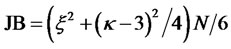 , where
  is the sample skewness,
  is the sample kurtosis, and
  is the sample size. Historical CMS data have been obtained from BloombergTM database.3
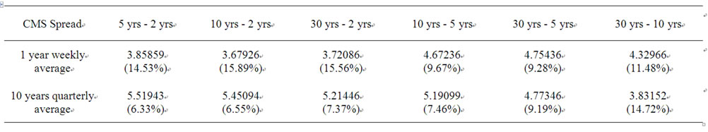
Table 1. JB statistics and associated p-values.
Table 1 presents the values of the statistics as results of the JB test.
The first row shows CMS spread rates for which the JB test has been done. The second row presents the test statistics results with their associated p-values when we use 1-year weekly average of CMS spread data—from 1 January 2007 to 31 December 2007. The third shows the test statistics results for 10-year quarterly average of CMS spread data—from 1 January 1998 to 31 December 2007. Overall, at 5 percent level of significance the normality assumption is accepted for each CMS spread and for both cases of the 1-year and the 10-year historical data. Based on this level of significance it is realistic to model the CMS spread rate as normally distributed in the valuation of both short and long maturity derivatives. The following section then proposes a Gaussian market models to value interest derivatives on CMS spread rates.
3. The Model
Let us consider a finite time horizon  in which trading is done. We assume the uncertainty in our economy is modeled by a complete filtered probability space,
 , in which
  is the set of all possible states of nature,
  is a filtration that satisfies the usual conditions and it is generated by two independent source of risk (two standard Brownian motions), and
  is a probability measure that belongs to
 , the class of equivalent probability measures on
 .
.
Let  be an increasing sequence of dates from which reset dates of financial derivatives will be taken.
  will denote the day-count fraction between times
  and
and . Let
. Let  be the price process of the risk-free discount bond paying one monetary unit at time
 . According to the asset pricing theory one can find a probability measure,
  , equivalent to
 , for which
  is the numeraire as in Geman et al. [6]. Following Jamshidian [7],
  will be called
  -forward measure.
At any given time , let us define
 to be the stochastic process of the forward CMS spread rate for the maturity date
 . Here
  denotes the view of investors at time
of whatwill be the level of the CMS spread rate at time . Because the value of the forward CMS spread rate can be either positive or negative, we assume its dynamics is driven by a Gaussian process. A martingale spread measure for this forward CMS spread exists. But as noticed by Antonov and Arneguy [8], the corresponding numeraire process for this measure is difficult to calculate. To overcome this difficulty, we define the dynamics of this forward CMS spread directly under the
  -forward measure as a Brownian motion with a drift. This drift arises from the convexity adjustment and the change of measure. Hence the stochastic differential equation of the forward CMS spread rate is represented as
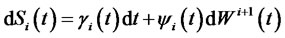 , (1)
, (1)
subject to the initial forward CMS spread rate , and where
  and
and  are deterministic bounded functions that are integrable and square integrable on
  respectively, and
  is a standard Brownian motion under the
  -forward measure.
At any given time  let us define
  to be the stochastic process of the
  -tenor forward LIBOR rate maturing at time
 . Here
  denotes the interest rate available at time
  for a risk-free loan which is effective at time
  and matures at time
 . As in the standard LIBOR market model, let us assume the dynamics of
  under the
  - forward measure to be a lognormal martingale.
It is important to note that under the  -forward measure if the forward LIBOR rate is driven only by the same source of risk that drives the forward CMS rate, both stochastic processes will be perfectly correlated, and hence it will be economically redundant to trade CMS spread derivatives, as investors can obtain the same result by trading the forward LIBOR rate. Therefore, we assume the forward LIBOR rate to be driven by an additional source of risk. This assumption has the implication that traders can have different views on the entire yield curve on the one hand and on the slope of a part of the yield curve on the other hand.4 The forward LIBOR rate is then assumed to be driven by the two Brownian motions and its dynamics under the
  -forward measure is given by the following stochastic differential equation
 , (2)
, (2)
subject to the initial forward LIBOR rate , and where
  is a deterministic bounded functions that is square integrable on
 , and
, and  is a standard Brownian motion under the
  -forward measure. This additional Brownian motion is independent of
 . The function
  is the correlation coefficient between
  and
and , and
, and
 is the orthogonal complement of
 .
.
Equation (1) defines the stochastic differential equation of the forward CMS spread rate under its relevant measure, the  -forward measure. This equation can lead to closed-form solutions to value financial derivatives that depend on a CMS spread rate at a single maturity date such as CMS spread caplets, floorlets, and digital options. However, for valuing financial derivatives that involve forward CMS spread rates at more than one maturity date, all rates needed to be modeled simultaneously, i.e., under a single measure as in the following proposition.
Proposition 1. Under the  -forward measure associated to the numeraire
 :
:
1) for , the expression of
  is given by Equation (1).
2) for ,
,
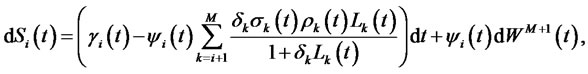 (3)
(3)
where
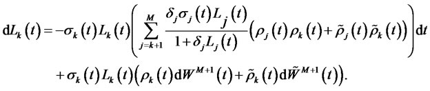 (4)
(4)
3) and for ,
,
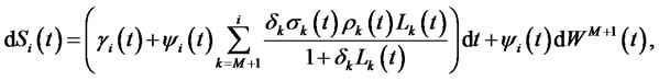 (5)
(5)
where
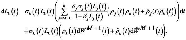 (6)
(6)
Proof:
Let us consider two consecutive forward LIBOR rate processes,  and
and , which their stochastic dynamics are described by Equation (2) under the
  -forward measure and the
  -forward measure respectively. It is straightforward to prove that by applying Ito’s lemma on the Radon-Nikodym derivative that allows the change of measure from the
  -forward measure to the
  -forward measure, and using Cameron-Martin-Girsanov theorem (as in e.g. Pelsser [9]) one obtain the following relationships
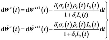
The result of the theorem is then obtained apply the above relationships repeatedly backward and forward on Equations (1) and (2).
4. A Numerical Example
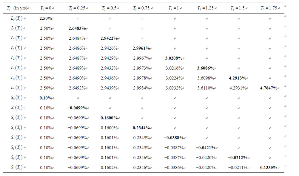
Table 2. Average of one thousand sample paths of forward LIBOR and forward CMS spread rates in the terminal measure with σ = 20%, ρ = 10%, ψ = 0.5%, γ = 0.1%, and δ = 0.25.
For illustration purpose,Table 2 shows the results of a one thousand paths of Monte Carlo simulation for generating forward LIBOR rates and forward CMS spread rates with a quarterly frequency over a two-year period. The results of this simulation can be used to valuing CMS spread derivatives that mature within two years and that involve forward CMS spread rates at more than one maturity date. This simulation is done under the terminal measure, i.e., the measure associated to the discount bond maturing in two years.
Although the CMS spread derivatives are increasing in popularity, they are still OTC instruments, and their market data are not easily available. Therefore, for simplicity of the illustration we assume all model parameters to be constant, i.e.,  ,
,  ,
,  ,
,  , and
, and . In the first column we consider the initial term structures of forward LIBOR and forward CMS spread rates to be flat. Even though we started the simulation with flat curves for both the forward LIBOR rates and the forward CMS spread rates, the end results shows that the expected forward LIBOR rates are increasing while the expected forward CMS spread rates are fluctuating around zero.
5. Closed-Form Solutions for CMS Spread Options
This section presents the derivation of closed-form solutions for valuing simple instruments which payoffs are functions of a CMS spread rate at a single maturity date, such as CMS spread caplets and floorlets. A CMS spread caplet (floorlet) is a call (put) option on a CMS spread rate. At maturity the buyer receives a payment from the seller if the CMS spread was above (below) the agreed strike rate. CMS spread caplets (floorlets) are not generally traded. However they are useful as they are building blocks of over-the-counter traded CMS spread caps (floors).
Let  be the price process of a caplet or a floorlet that resets at time
  and pays off at time
  with a strike rate
 . We have
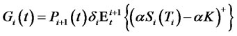 ,
,
where  for caplet and floorlet respectively, and
  represents the expectation with respect to the
  -forward measure and the sigma-algebra
 .
.
Thestochastic differential equation of the forward CMS spread in Equation (1) implies
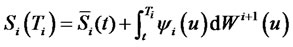 , (8)
, (8)
where 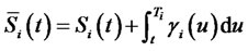 is the convexity adjusted forward CMS spread for the maturity
 , as seen at time
 . Note that the second term of the right hand side of Equation (8) is normally distributed, as it is a stochastic integral of a deterministic function times a Brownian motion. Hence
  is normally distributed with mean
  as the Ito integral is a martingale, and variance
 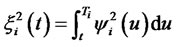 by Ito’s isometry. ThusEquation (7) can be rewritten as
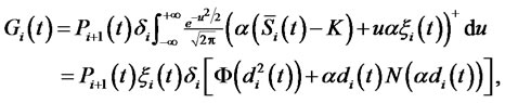
where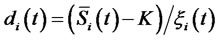 , and
, and  and
and  are the standard normal density and cumulative distribution functions respectively.
Another important CMS spread option is the digital option. It is an instrument in which, at maturity, the holder receives a payment if the CMS spread crosses a certain barrier level. CMS spread digital options are not generally traded. However they are useful as they are building blocks of range accrual CMS spread notes that are over-the-counter traded. If 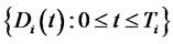 represents the price process of a digital option that pays one monetary unit at time
  in case the CMS spread rate is greater or less than a strike rate
  at time
  , then
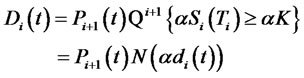 ,
,where  if the CMS spread is greater than and less than the strike respectively, and
  is given in Equation (9).
6. Concluding Remarks
We proposed a two-factor model for valuing CMS spread derivatives assuming the CMS spread rate is driven by one of the risk sources that drive the LIBOR rate. Our proposed model is simultaneously calibrated to LIBOR instruments and CMS spread instruments and is flexible enough to take into account various deterministic volatility and convexity adjustment functions. Furthermore, this model is easy to implement, and can be used to value Constant Maturity Treasury (CMT) spread derivatives. An area of improvement would be to show the consistency between the forward LIBOR rates and the forward CMS spread rates.
REFERENCES
- Fannie Mae, “Fannie Mae Universal Debt Facility,” Federal Home Loan Association, Washington DC, 2008. http://www.fanniemae.com/markets/debt/pdf/CUSIP_PS31398ANE8.pdf
- R. Carmona and V. Durrleman, “Pricing and Hedging of Spread Options,” SIAM Review, Vol. 45, No. 4, 2003, pp. 627-685. doi:10.1137/S0036144503424798
- D. Belomestny, A. Kolodko and J. Schoenmakers, “Pricing Spreads in the Libor Market Model,” Weierstrass Institute for Applied Analysis and Stochastics, Berlin, 2008.
- M. Lutz and R. Kiesel, “Efficient Pricing of CMS Spread Options in a Stochastic Volatility LMM,” Institute of Mathematical Finance, Ulm University, Ulm, 2010.
- W. Margrabe, “The Value of an Option to Exchange One Asset for the Another,” Journal of Finance, Vol. 33, No. 1, 1978, pp. 177-186. doi:10.2307/2326358
- H. Geman, N. Karoui and J. C. Rochet, “Change of Numeraire, Change of Probability Measure and Option Pricing,” Journal of Applied Probability, Vol. 32, No. 2, 1995, pp. 443-458. doi:10.2307/3215299
- F. Jamshidian, “Bond and Option Evaluation in the Gaussian Interest Rate Model,” Research in Finance, Vol. 9, 1991, pp. 131-170.
- A. V. Antonov and M. Arneguy, “Analytical Formulas for Pricing CMS Products in the Libor Market Model with Stochastic Volatility,” Numerix Software Ltd., London, 2009.
- A. Pelsser, “Efficient Methods for Valuing Interest Rate Derivative,” Springer-Verlag, New York, 2000.
NOTES
*
The views expressed herein are the author’s and should not be interpreted as reflecting those of the US Department of the Treasury.1Fannie Mae previously issued a 10-year CMS spread 10 yrs - 2 yrs effective on 25th July 2007, and a 15-year CMS spread 30 yrs - 2 yrs effective on 23rd January 2008 under the bond CUSIP 31398AEQ1 and 31398ALA8 respectively.
3The CMS tickers are represented as USSWAPyy, where yy is the year indicator. For Example the tickers for CMS 30 yrs and CMS 2 yrs are USSWAP30 and USSWAP02 respectively.
4This will be illustrated in the numerical example.