ABSTRACT

A continuous random variable is expanded as a sum of a sequence of uncorrelated random variables. These variables are principal dimensions in continuous scaling on a distance function, as an extension of classic scaling on a distance matrix. For a particular distance, these dimensions are principal components. Then some properties are studied and an inequality is obtained. Diagonal expansions are considered from the same continuous scaling point of view, by means of the chi-square distance. The geometric dimension of a bivariate distribution is defined and illustrated with copulas. It is shown that the dimension can have the power of continuum.

Keywords: Statistical Distances; Orthogonal Expansions; Principal Directions of Random Variables; Diagonal Expansions; Copulas; Uncountable Dimensionality

1. Introduction

Let be a random variable on a probability space with range, absolutely continuous cdf and density w.r.t. the Lebesgue measure. Our main purpose is to expand (a function of) as

(1)

where is a sequence of uncorrelated random variables, which can be seen as a decomposition of the so-called geometric variability defined below, a dispersion measure of in relation with a suitable distance function Here orthogonality is synonymous with a lack of correlation.

Some goodness-of-fit statistics, which can be expressed as integrals of the empirical processes of a sample, have expansions of this kind [1-3]. Expansion (1) is obtained following a similar procedure, except that we have a sequence of uncorrelated rather than independent random variables. Finite orthogonal expansions appear in analysis of variance and in factor analysis. Orthogonal expansions and series also appear in the theory of stochastic processes, in martingales in the wide sense ([4], Chap. 4; [5], Chap. 10), in non-parametric statistics [6], in goodness-of-fit tests [7,8], in testing independence [9] and in characterizing distributions [10].

The existence of an orthogonal expansion and some classical expansions is presented in Section 2. A continuous extension of matrix formulations in multidimensional scaling (MDS), which provides a wide class of expansions, is presented in Section 3. Some interesting expansions are obtained in Section 4 for a particular distance as well as additional results, such as an optimal property of the first dimension. Section 5 contains an inequality concerning the variance of a function. Section 6 is devoted to diagonal expansions from the continuous scaling point of view. Sections 7 and 8 are devoted to canonical correlation analysis, including a continuous generalization. This paper extends the previous results on continuous scaling [11-14], and other related topics [15,16].

2. Existence and Classical Expansions

There are many ways of obtaining expansion (1). Our aim is to obtain some explicit expansions with good properties from a multivariate analysis point of view. However, before doing this, let us prove that a such expansion exists and present some classical expansions.

Theorem 1. Let be an absolutely continuous r.v. with density and support and a measurable function such that and Then there exists a sequence of uncorrelated r.v.’s such that

(2)

with where the series converges in the mean square as well as almost surely.

Proof. Consider the Lebesgue spaces and of measurable functions on such that and respectively. Obviously, and are separable Hilbert spaces with quadratic-norms and, respectively. Moreover given by

is a linear isometry of onto i.e.,

Let be an orthonormal basis for. Accordingly, given by

is an orthonormal basis for. The assumption, together with, is equivalent to. In fact, Hence where are the Fourier coefficients and Letting we deduce that, where the series converges in and where is Kronecker’s delta. Replacing by, and defining, we obtain

This series converges almost surely, since the series converges in We may suppose Next, for, we have cov as asserted. Finally, note that In particular, the series in (2) converges also in the mean square. W Some classical expansions for or a function of are next given.

2.1. Legendre Expansions

Let be the cdf of An all-purpose expansion can be obtained from the shifted Legendre polynomials on where The first three are

Note that Thus we may consider the orthogonal expansion

where and are the Fourier coefficients. This expansion is quite useful due to the simplicity of these polynomials, is optimal for the logistic distribution, but may be improved for other distributions, as it is shown below.

2.2. Univariate Expansions

A class of orthogonal expansions arises from

(3)

where both are probability density functions. Then is a complete orthonormal set w.r.t.

2.3. Diagonal Expansions

Lancaster [17] studied the orthogonal expansions

(4)

where is a bivariate probability density with marginal densities Then are complete orthonormal sets w.r.t and respectively. Moreover and

where is the n-th canonical correlation between and

Expansion (4) can be viewed as a particular extension of Theorem 3, proved below, when the distance is the so-called chi-square distance. This is proved in [18]. See Section 6.

3. Continuous Scaling Expansions

In this section we propose a distance-based approach for obtaining orthogonal expansions for a r.v., which contains the Karhunen-Loève expansion of a Bernoulli process related to as a particular case. We will prove that we can obtain suitable expansions using continuous multidimensional scaling on a Euclidean distance.

Let be a dissimilarity function, i.e., and for all

Definition 1. We say that is a Euclidean distance function if there exists an embedding

where is a real separable Hilbert space with quadratic norm, such that

We may always view the Hilbert space as a closed linear subspace of In this case, we may identify with where for is a vector in Accordingly, for

(5)

Definition 2. is called a Euclidean configuration to represent The geometric variability of w.r.t. is defined by

The proximity function of to is defined by

(6)

The double-centered inner product related to is the symmetric function

(7)

These definitions can easily be extended to random vectors. For example, if is is an observation of and is the Euclidean distance in, then and

is the Mahalanobis distance from to

The function is symmetric, semi-definite positive and satisfies

(8)

It can be proved [19], that there is an embedding of into such that

G is the continuous counterpart of the centered inner product matrix computed from a distance matrix and used in metric multidimensional scaling [20,21]. The Euclidean embedding or method of finding the Euclidean coordinates from the Euclidean distances was first given by Schoenberg [22]. The concepts of geometric variability and proximity function, were originated in [23] and are used in discriminant analysis [19], and in constructing probability densities from distances [24]. In fact, is a variant of Rao’s quadratic entropy [25]. See also [14,26].

In order to obtain expansions, our interest is on and i.e., we substitute by the r.v.

For convenience and analogy with the finite classic scaling, let us use a generalized product matrix notation (i.e., a “multivariate analysis notation”), following [18]. We write as where is a Euclidean centered configuration to represent according to (5), (8), i.e., we substitute by in and suppose that each has mean 0. The covariance matrix of is where for and may be expressed as

where stands for the continuous diagonal matrix and the row × column multiplication, denoted by is evaluated at and then follows an integration w.r.t.

In the theorems below, and stands for and

Theorem 2. Suppose that for a Euclidean distance the geometric variability is finite. Define Then:

1.

2. is a Hilbert-Schmidt kernel, i.e.,

Proof. Let be i.i.d. and write From (7) and hence using (8),

This proves 1). Next, is p.s.d., so for the matrix with entries is p.s.d. In particular, for with the determinant

is non-negative. Thus

Integrating this inequality over gives

and 2) is also proved. W Theorem 3. Suppose that for a Euclidean distance is finite. Then the kernel admits the expansion

(9)

where is a complete orthonormal set of eigenfunctions in. Let

(10)

and Then and is a sequence of centered and uncorrelated r.v.’s, which are principal components of where and

Proof. The eigendecomposition (9) exists because is a Hilbert-Schmidt kernel and by Theorem 2. Next, (9) and (10) can be written as

(11)

i.e., and where Thus, for all

Next, for we have In particular, since

we have Moreover, from (10) we also have

where is Kronecker’s delta, showing that the variables are centered and uncorrelated.

Recall the product matrix notation. The principal components of such that are where

(12)

is the spectral decomposition of Premultiplying (12) by and postmultiplying by we obtain and therefore

Thus the columns of are eigenfunctions of This shows that see

(11), and contains the principal components of The rows in may be accordingly called the principal coordinates of distance. This name can be justified as follows.

Let us write the coordinates and suppose that is another Euclidean configurations giving the same distance. The linear transformation is orthogonal and with Then the r.v.’s are uncorrelated and

Thus is the first principal coordinate in the sense that is maximum. The second coordinate is orthogonal to and has maximum variance, and so on with the others coordinates. W The following expansions hold as an immediate consequence of this theorem:

(13)

(14)

(15)

where and , with are sequences of centered and uncorrelated random variables, which are principal components of. We next obtain some concrete expansions.

4. A Particular Expansion

If is a continuous r.v. with finite mean and variance, say, and is the ordinary Euclidean distance, then it is easy to prove that

Then from (14) and taking we obtain which provides the trivial expansion A much more interesting expansion can be obtained by taking the square root of.

4.1. The Square Root Distance

Let us consider the distance function

(16)

The double-centered inner product is next given.

Definition 3. Let be defined as where is defined in (10).

We immediately have the following result.

Proposition 1. The function satisfies:

1.

2.

3.

Proposition 2. Assuming i.i.d., if, then

(17)

Proof. From and combining (7) and (6), we obtain

where which satisfies Hence and (17) holds. W Proposition 3. The following expansion holds

(18)

Proof. Using (17) and expanding and setting we get (18). W Replacing by we have the expansion

(19)

and, as a consequence [12]:

where is distributed as and This expansion also follows from (15).

If from (19) we can also obtain the expansions

(20)

as well as

(21)

where the convergence is in the mean square sense [27].

4.2. Principal Components

Related to the r.v. with cdf let us define the stochastic process where is the indicator of and follows the Bernoulli distribution with. For the distance (16), the relation between, the Bernoulli process and is

(22)

where and is a realization of X. Thus X is a continuous configuration for Note that, if is finite, then

The covariance kernel of X is given by Let us consider the integral operator with kernel

where is an integrable function on Let be the countable orthonormal set of eigenfunctions of i.e., We may suppose that constitutes a basis of and the eigenvalues are arranged in descending order. As a consequence of Mercer’s theorem, the covariance kernel can be expanded as

(23)

Theorem 4. The functions (see definition 3), satisfy:

1.

2. is a countable set of uncorrelated r.v.’s such that

3. are principal coordinates for the distance i.e.,

Proof. To prove 1), let us use the multiplication “*” and write as where

i.e., with where if and 0 otherwise. Then is a centered continuous configuration for and clearly Arguing as in Theorem 3, the centered principal coordinates are i.e.,

2) is a consequence of Theorem 3. An alternative proof follows by taking in the formula for the covariance [28]:

(24)

where See Theorem 6.

To prove 3), let and Then and see (22), is

This proves that are principal coordinates for the distance W The above results have been obtained via continuous scaling. For this particular distance, we get the same results by using the Karhunen-Loève (also called Kac-Siegert) expansion of X, namely,

(25)

where i.e., Thus each is a principal component of X and the sequence constitutes a countable set of uncorrelated random variables.

4.3. The Differential Equation

Let where It can be proved [12] that the means eigenvalues and functions satisfy the second order differential equation

(26)

The solution of this equation is well-known when is uniform.

Examples of eigenfunctions principal components and the corresponding variances are [12,27,29]:

1. is uniform:

2. is exponential with unit mean. If

where is the n-th positive root of and are the Bessel functions of the first order.

3. is standard logistic If

(27)

where are the shifted Legendre polynomials on

4. is Pareto with

where

and

Note that the change of variable transforms in and (26) in

Hence and providing solutions for the variable For instance, we immediately can obtain the principal dimensions of the Pareto distribution with cdf

4.4. A Comparison

The results obtained in the previous sections can be compared and summarized in Table 1, where is a random variable with absolutely continuous cdf density and support The continuous scaling expansion is found w.r.t. the distance (16). Note that we reach the same orthogonal expansions (we only include two), but this continuous scaling approach is more general, since by changing the distance we may find other

principal directions and expansions. This distance-based approach may be an alternative to the problem of finding nonlinear principal dimensions [30].

4.5. Some Properties of the Eigenfunctions

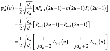
In this section we study some properties of the eigenfunctions and their integrals

Proposition 4. The first eigenfunction is strictly positive and satisfies

Proof. is positive, so is also positive (Perron-Frobenius theorem). On the other hand

which satisfies W Clearly, if is positive, is increasing and positive. Moreover, any satisfies the following bound.

Proposition 5. If is finite then is also finite and

(28)

Proof. is an eigenfunction and from (24)

Hence W Proposition 6. The principal components of constitutes a complete orthogonal system of

Proof. The orthogonality has been proved as a consequence of (24). Let be a continuous function such that Suppose that exists. As is a complete system and integrating, we have But which shows that must be constant. W

4.6. The First Principal Component

In this section we prove two interesting properties of and the first principal component see [10].

Proposition 7. The increasing function characterizes the distribution of

Proof. Write Then satisfies the differential equation (see (26))

(29)

where When the function is given, and may be obtained by solving the equations

and the density of is W Proposition 8. For a fixed let denote the squared correlation between and a function The average of weighted by is maximum for i.e.,

Proof. Let us write (see Proposition 6) Then and we can suppose From (25)

As we have

Thus the supreme is attained at W

5. An Inequality

The following inequality holds for with the normal distribution [31,32]:

where is an absolutely continuous function and has finite variance. This inequality has been extended to other distributions by Klaassen [33]. Let us prove a related inequality concerning the function of a random variable and its derivative.

If is the first principal dimension, then and We can define the probability density with support given by

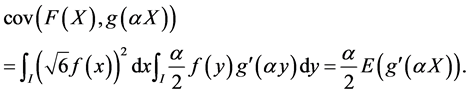
Theorem 5. Let be a r.v. with pdf If is an absolutely continuous function and has finite variance, the following inequality holds

(30)

with equality if is

Proof. From Proposition 6, we can write where Then and, so

From Parseval’s identity Thus we have

proving (30). Moreover, if we have and W Inequality (30) is equivalent to

(31)

Some examples are next given.

5.1. Uniform Distribution

Suppose uniform Then and We obtain

5.2. Exponential Distribution

Suppose exponential with mean 1. Then and

where satisfies Inequality (31) is

where

5.3. Pareto Distribution

Suppose with density for Then and

where satisfies Inequality (31) is

where

5.4. Logistic Distribution

Suppose that follows the standard logistic distribution. The cdf is

and the density is

This distribution has especial interest, as the two first principal components are i.e., proportional to the cdf and the density, respectively. Note that can be obtained directly, as if we write then and (29) gives

so Similarly, we can obtain Besides

i.e., the expectation of w.r.t. with density is maximum for

Now and The density is just, therefore inequality (30) for the logistic distribution reduces to

In general, if is logistic with variance then with Noting that the functions are orthogonal to and using (24), we obtain

As the Cauchy-Schwarz inequality proves that

6. Diagonal Expansions

Correspondence analysis is a variant of multidimensional scaling, used for representing the rows and columns of a contingency table, as points in a space of low-dimension separated by the chi-square distance. See [15,34]. This method employs a singular value decomposition (SVD) of a transformed matrix. A continuous scaling expansion, viewed as a generalization of correspondence analysis, can be obtained from (3) and (4).

6.1. Univariate Case

Let be two densities with the same support Define the squared distance

The double-centered inner product is given by

and the geometric variability is

which is a Pearson measure of divergence between and If is an orthonormal basis for we may consider the expansion

and defining then

and

However, are not the principal coordinates related to the above distance. In fact, the continuous scaling dimension is 1 for this distance and it can be found in a straightforward way.

6.2. Bivariate Case

Let us write (4) as

(32)

where are the canonical functions and is the sequence of canonical correlations. Note that and

Suppose that is absolutely continuous w.r.t. and let us consider the Radom-Nikodym derivative

The so-called chi-square distance between is given by

Let the Pearson contingency coefficient is defined by

The geometric variability of the chi-square distance is In fact

The proximity function is

and the double-centered inner product is

We can express (32) as

This SVD exists provided that Multiplying by himself and integrating w.r.t. we readily obtain

Comparing with (9) we have the principal coordinates where which satisfy

Then

See [18] for further details.

Finally, the following expansion in terms of cdf’s holds [35]:

(33)

where Using a matrix notation, this diagonal expansion can be written as

where stands for the diagonal matrix with the canonical correlations, and

7. The Covariance between Two Functions

Here we generalize the well-known Hoeffding’s formula

which provides the covariance in terms of the bivariate and univariate cdf’s. The proof of the generalization below uses Fubini’s theorem and integration by parts, being different from the proof given in [28].

Let us suppose that the supports of are the intervals respectively, although the results may also hold for other subsets of We then have

Theorem 6. If are two functions defined on respectively, such that:

1. Both functions are of bounded variation.

2.

3. The expectations are finite.

Then:

(34)

Proof. The covariance exists and is

where Integration by parts gives

and similarly By Fubini’s theorem for transition probabilities

where is the cdf of given, we can write

We first integrate with respect to Setting to find integration by parts gives

Since setting we find

and setting again integration by parts gives

where Therefore

A last simplification shows that W

8. Canonical Analysis

Given two sets of variables, the purpose of canonical correlation analysis is to find sets of linear combinations with maximal correlation. In Section 6.2 we studied, from a multidimensional scaling perspective, the nonlinear canonical functions of and with joint pdf Here we find the canonical correlations and functions for several copulas.

Let be a bivariate random vector with cdf, where and are uniform. Then is a cdf called copula [36]. Let us suppose symmetric. Then Therefore, in finding the canonical functions, we can suppose

Let us consider the symmetric kernels

We seek the canonical functions and the corresponding canonical correlations, i.e.,

(35)

Definition 4. A generalized eigenfuction of w.r.t. with eigenvalue is a function such that

(36)

From the theory of integral equations, we have

(37)

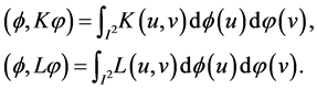
Definition 5. On the set of functions in with we define the inner products

Clearly, see Theorem 6, if is eigenfunction of w.r.t. with eigenvalue we have the covariance and the variance Therefore the correlation between is:

Thus the canonical correlations of are the eigenvalues of w.r.t.

Justified by the embedding in a Euclidean or Hilbert space via the chi-square distance, the geometric dimension of a copula is defined as the cardinal of the set of canonical correlations. The dimension can be finite, infinite countable (cardinality of) or uncountable (cardinality of the continuum).

We next illustrate these results with some copulas. Since is a copula, the so-called FréchetHoeffding upper bound, we firstly suggest a procedure for constructing copulas and performing canonical analysis. This procedure is based on the expansion (23) for the logistic distribution.

For this distribution, if we have [27]:

where is given in (27). With the change we find:

(38)

with and

where are Legendre polynomials and are shifted Legendre polynomials on. Thus etc.

8.1. FGM Copula

If we consider only in (38), we obtain the Farlie-Gumbel-Morgenstern copula:

Then and if Thus is an eigenfunction with eigenvalue Then and are the canonical functions with canonical correlation The geometric dimension is one.

8.2. Extended FGM Copula

By taking more terms in expansion (38), we may consider the following copula

where The canonical correlations are The canonical functions are respectively. This copula has dimension 3.

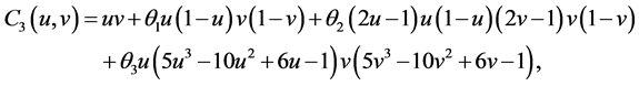
Clearly reduces to the FGM copula if When the dimension is 2, i.e., we have a copula with cubic sections [37]. A generalization is given in [38].

8.3. Cuadras-Augé Copula

The Cuadras-Augé family of copulas [39] is defined as the weighted geometric mean of and

For this copula, the canonical correlations constitute a continuous set. If for and 0 otherwise, it can be proved [40] that the set of eigenpairs of w.r.t. is given by

Thus, the set of canonical functions and correlations for the Cuadras-Augé copula is the uncountable set with dimension of the power of the continuum. In particular, the maximum correlation is the parameter with canonical function the Heaviside distribution The maximum correlation was obtained by Cuadras [28].

[1] REFERENCES

[2] T. W. Anderson and M. A. Stephens, “The Continuous and Discrete Brownian Bridges: Representation and Applications,” Linear Algebra and Its Applications, Vol. 264, 1996, pp. 145-171. http://dx.doi.org/10.1016/S0024-3795(97)00015-3

[3] J. Durbin and M. Knott, “Components of Cramér-von Mises Statistics. I,” Journal of the Royal Statistical Society: Series B, Vol. 34, 1972, pp. 290-307.

[4] J. Fortiana and C. M. Cuadras, “A Family of Matrices, the Discretized Brownian Bridges and Distance-Based Regression,” Linear Algebra and Its Applications, Vol. 264, 1997, pp. 173-188. http://dx.doi.org/10.1016/S0024-3795(97)00051-7

[5] J. L. Doob, “Stochastic Processes,” Wiley, New York, 1953.

[6] M. Loève, “Probability Theory,” 3rd Edition, Van Nostrand, Princeton, 1963.

[7] G. K. Eagleson, “Orthogonal Expansions and U-Statistics,” Australian Journal of Statistics, Vol. 21, No. 3, 1979, pp. 221-237. http://dx.doi.org/10.1111/j.1467-842X.1979.tb01141.x

[8] C. M. Cuadras and D. Cuadras, “Orthogonal Expansions and Distinction between Logistic and Normal,” In: C. Huber-Carol, N. Balakrishnan, M. S. Nikulin and M. Mesbah, Eds., Goodness-Of-Fit Tests and Model Validity, Birkhäuser, Boston, 2002, pp. 327-339. http://dx.doi.org/10.1007/978-1-4612-0103-8_24

[9] J. Fortiana and A. Grané, “Goodness-Of-Fit Tests Based on Maximum Correlations and Their Orthogonal Decompositions,” Journal of the Royal Statistical Society: Series B, Vol. 65, No. 1, 2003, pp. 115-126. http://dx.doi.org/10.1111/1467-9868.00375

[10]  C. M. Cuadras, “Diagonal Distributions via Orthogonal Expansions and Tests of Independence,” In: C. M. Cuadras, J. Fortiana and J. A. Rodriguez-Lallena, Eds., Distributions with Given Marginals and Statistical Modelling, Kluwer Academic Press, Dordrecht, 2002, pp. 35-42. http://dx.doi.org/10.1007/978-94-017-0061-0_5

[11]  C. M. Cuadras, “First Principal Component Characterization of a Continuous Random Variable,” In: N. Balakrishnan, I. G. Bairamov and O. L. Gebizlioglu, Eds., Advances on Models, Characterizations and Applications, Chapman and Hall/CRC, London, 2005, pp. 189-199. http://dx.doi.org/10.1201/9781420028690.ch12

[12]  C. M. Cuadras and J. Fortiana, “Continuous Metric Scaling and Prediction,” In: C. M. Cuadras and C. R. Rao, Eds., Multivariate Analysis, Future Directions 2, Elsevier Science Publishers B. V. (North-Holland), Amsterdam, 1993, pp. 47-66.

[13]  C. M. Cuadras and J. Fortiana, “A Continuous Metric Scaling Solution for a Random Variable,” Journal of Multivariate Analysis, Vol. 52, No. 1, 1995, pp. 1-14. http://www.sciencedirect.com/science/article/pii/S0047259X85710019 http://dx.doi.org/10.1006/jmva.1995.1001

[14]  C. M. Cuadras and J. Fortiana, “Weighted Continuous Metric Scaling,” In: A. K. Gupta and V. L. Girko, Eds., Multidimensional Statistical Analysis and Theory of Random Matrices, VSP, Zeist, 1996, pp. 27-40.

[15]  C. M. Cuadras and J. Fortiana, “The Importance of Geometry in Multivariate Analysis and Some Applications,” In: C. R. Rao and G. Szekely, Eds., Statistics for the 21st Century, Marcel Dekker, New York, 2000, pp. 93-108.

[16]  C. M. Cuadras and D. Cuadras, “A Parametric Approach to Correspondence Analysis,” Linear Algebra and Its Applications, Vol. 417, No. 1, 2006, pp. 64-74. http://www.sciencedirect.com/science/article/pii/S0024379505005203 http://dx.doi.org/10.1016/j.laa.2005.10.029

[17]  C. M. Cuadras and D. Cuadras, “Eigenanalysis on a Bivariate Covariance Kernel,” Journal of Multivariate Analysis, Vol. 99, No. 10, 2008, pp. 2497-2507. http://www.sciencedirect.com/science/article/pii/S0047259X08000754 http://dx.doi.org/10.1016/j.jmva.2008.02.039

[18]  H. O. Lancaster, “The Chi-Squared Distribution,” Wiley, New York, 1969.

[19]  C. M. Cuadras, J. Fortiana and M. J. Greenacre, “Continuous Extensions of Matrix Formulations in Correspondence Analysis, with Applications to the FGM Family of Distributions,” In: R. D. H. Heijmans, D. S. G. Pollock and A. Satorra, Eds., Innovations in Multivariate Statistical Analysis, Kluwer Academic Publisher, Dordrecht, 2000, pp. 101-116. http://dx.doi.org/10.1007/978-1-4615-4603-0_7

[20]  C. M. Cuadras, J. Fortiana and F. Oliva, “The Proximity of an Individual to a Population with Applications in Discriminant Analysis,” Journal of Classification, Vol. 14, No. 1, 1997, pp. 117-136. http://dx.doi.org/10.1007/s003579900006

[21]  K. V. Mardia, J. T. Kent and J. M. Bibby, “Multivariate Analysis,” Academic Press, London, 1979.

[22]  T. F. Cox and M. A. Cox, “Multidimensional Scaling,” Chapman and Hall, London, 1994.

[23]  I. J. Schoenberg, “Remarks to Maurice Fréchet’s Article ‘Sur la définition axiomtique d’une classe d’espaces vectoriels distanciés applicables vectoriellment sur l’espace de Hilbert’,” Annals of Mathematics, Vol. 36, No. 3, 1935, pp. 724-732. http://dx.doi.org/10.2307/1968654

[24]  C. M. Cuadras, “Distance Analysis in Discrimination and Classification Using Both Continuous and Categorical Variables,” In: Y. Dodge, Ed., Statistical Data Analysis and Inference, Elsevier Science Publishers B. V. (North-Holland), Amsterdam, 1989, pp. 459-473.

[25]  C. M. Cuadras, E. A. Atkinson and J. Fortiana, “Probability Densities from Distances and Discriminant Analysis,” Statistics and Probability Letters, Vol. 33, No. 4, 1997, pp. 405-411. http://dx.doi.org/10.1016/S0167-7152(96)00154-X

[26]  C. R. Rao, “Diversity: Its Measurement, Decomposition, Apportionment and Analysis,” Sankhyā: The Indian Journal of Statistics, Series A, Vol. 44, No. 1, 1982, pp. 1-21.

[27]  Z. Liu and C. R. Rao, “Asymptotic Distribution of Statistics Based on Quadratic Entropy and Bootstrapping,” Journal of Statistical Planning and Inference, Vol. 43, No. 1-2, 1995, pp. 1-18. http://dx.doi.org/10.1016/0378-3758(94)00005-G

[28]  C. M. Cuadras and Y. Lahlou, “Some Orthogonal Expansions for the Logistic Distribution,” Communications in Statistics— Theory and Methods, Vol. 29, No. 12, 2000, pp. 2643-2663. http://dx.doi.org/10.1080/03610920008832629

[29]  C. M. Cuadras, “On the Covariance between Functions,” Journal of Multivariate Analysis, Vol. 81, No. 1, 2002, pp. 19-27. http://www.sciencedirect.com/science/article/pii/S0047259X01920007 http://dx.doi.org/10.1006/jmva.2001.2000

[30]  C. M. Cuadras and Y. Lahlou, “Principal Components of the Pareto Distribution,” In: C. M. Cuadras, J. Fortiana and J. A. Rodriguez-Lallena, Eds., Distributions with Given Marginals and Statistical Modelling, Kluwer Academic Press, Dordrecht, 2002, pp. 43-50. http://dx.doi.org/10.1007/978-94-017-0061-0_6

[31]  E. Salinelli, “Nonlinear Principal Components, II: Characterization of Normal Distributions,” Journal of Multivariate Analysis, Vol. 100, No. 4, 2009, pp. 652-660. http://dx.doi.org/10.1016/j.jmva.2008.07.001

[32]  H. Chernoff, “A Note on an Inequality Involving the Normal Distribution,” Annals of Probability, Vol. 9, No. 3, 1981, pp. 533-535. http://dx.doi.org/10.1214/aop/1176994428

[33]  T. Cacoullos, “On Upper and Lower Bounds for the Variance of a Function of a Random Variable,” Annals of Probability, Vol. 10, No. 3, 1982. pp. 799-809. http://dx.doi.org/10.1214/aop/1176993788

[34]  C. A. J. Klaassen, “On an Inequality of Chernoff,” Annals of Probability, Vol. 13, No. 3, 1985, pp. 966-974. http://dx.doi.org/10.1214/aop/1176992917

[35]  M. J. Greenacre, “Theory and Applications of Correspondence Analysis,” Academic Press, London, 1984.

[36]  C. M. Cuadras, “Correspondence Analysis and Diagonal Expansions in Terms of Distribution Functions,” Journal of Statistical Planning and Inference, Vol. 103, No. 1-2, 2002, pp. 137-150. http://dx.doi.org/10.1016/S0378-3758(01)00216-6

[37]  R. B. Nelsen, “An Introduction to Copulas,” 2nd Edition, Springer, New York, 2006.

[38]  R. B. Nelsen, J. J. Quesada-Molina and J. A. Rodriguez-Lallena, “Bivariate Copulas with Cubic Sections,” Journal of Nonparametric Statistics, Vol. 7, No. 3, 1997, pp. 205-220. http://dx.doi.org/10.1080/10485259708832700

[39]  C. M. Cuadras and W. Daz, “Another Generalization of the Bivariate FGM Distribution with Two-Dimensional Extensions,” Acta et Commentationes Universitatis Tartuensis de Mathematica, Vol. 16, No. 1, 2012, pp. 3-12. http://math.ut.ee/acta/16-1/CuadrasDiaz.pdf

[40]  C. M. Cuadras and J. Augé, “A Continuous General Multivariate Distribution and Its Properties,” Communications in Statistics—Theory and Methods, Vol. 10, No. 4, 1981, pp. 339-353. http://dx.doi.org/10.1080/03610928108828042

[41]  C. M. Cuadras, “Continuous Canonical Correlation Analysis,” Research Letters in the Information and Mathematical Sciences, Vol. 8, 2005, pp. 97-103. http://muir.massey.ac.nz/handle/10179/4454