Open Journal of Statistics
Vol.1 No.2(2011), Article ID:6347,6 pages DOI:10.4236/ojs.2011.12009
Moved Score Confidence Intervals for Means of Discrete Distributions
Department of Statistics, Zhejiang A & F University, Lin’an, Zhejiang, China
E-mail: guanyu@zafu.edu.cn
Received April 23, 2011; revised May 15, 2011; accepted May 21, 2011
Keywords: Confidence Interval, Confidence Level, Coverage Probability, Discrete Distribution, Moved Score Confidence Interval
Abstract
Let X denote a discrete distribution as Poisson, binomial or negative binomial variable. The score confidence interval for the mean of X is obtained based on inverting the hypothesis test and the central limit theorem is discussed and recommended widely. But it has sharp downward spikes for small means. This paper proposes to move the score interval left a little (about 0.04 unit), called by moved score confidence interval. Numerical computation and Edgeworth expansion show that the moved score interval is analogous to the score interval completely and behaves better for moderate means; for small means the moved interval raises the infimum of the coverage probability and improves the sharp spikes significantly. Especially, it has unified explicit formulations to compute easily.
1. Introduction
Forming a confidence interval (CI) for the mean of a discrete distribution is one of the most basic problems in statistics, since the discrete lattice nature and skewness make the problem complicated. Let X be a discrete variable with the mean E(X) = μ and the variance Var(X) = aμ + bμ2. For X~π (λ) Poisson distribution with mean λ, a = 1, b = 0; for X~B(n, p) binomial distribution with mean np, a = 1, b = –1/n; for X~NB(r,p) negative binomial distribution, mean rp/q, a = 1, b = 1/r. Where q = 1 – p.
It is well known that the normal distribution N(μ, aμ + bμ2) could be regarded as an approximation to X for large sample by the central limit theorem. Let
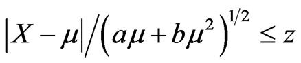 , where
  is the
  th percentile of the standard normal distribution. We have the score confidence interval for the mean μ as follows
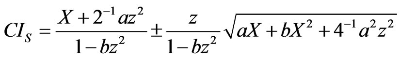 .
.
The score interval is an approximate interval and has many better properties for moderate mean μ. Those articles concern approximate confidence interval almost refer to the score interval. See references in this paper.
The exact confidence interval for the mean and the confidence level 1 – α is obtained by solving equations 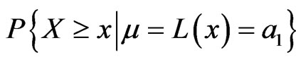 and
and , where α1 + α2 = α.
In this paper, the exact confidence interval indicates the shortest length interval with less coverage probability not less than the nominal level (see [1]). Obviously, the exact interval has not explicit formulation and its computation will be troublesome if one does not use a computer. In general, an approximate interval cannot guarantee its coverage probabilities all not less than the nominal level, but its formula is simple and easily computed [2-5].
This paper discusses a moved score interval CI(c) for the means of Poisson, binomial and negative binomial variables. CI(c) with its coverage probability is introduced in section 2. From section 3 to section 4, CI(c) for the means of Poisson, binomial, negative binomial variables are discussed respectively. In section 5, Edgeworth expansion on coverage probabilities of CI(c) are investigated and compared. Conclusion and recommendation appears in the last section.
2. Moved Score Confidence Interval
Let X be a variable with the mean μ and the variance aμ + bμ2. A moved score confidence interval for the mean μ is defined as

Obviously, CI(c) is equivalent to moving CI(1/2) = CIS left 1/2 – c units.
Theorem 1 The coverage probability of CI(c) can be computed as
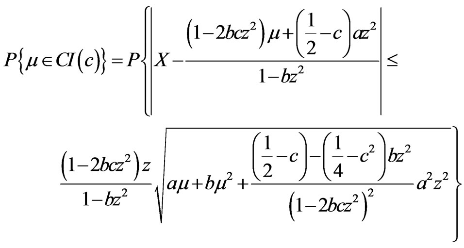
Proof Let
 . By some trivial deduction, the formula is obtained easily.
Following theorem is the specific case of theorem 1.
Theorem 2 1) If X~π (λ), the moved score interval on the mean is defined as
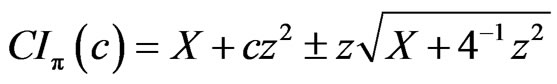
and its coverage probability is equal to
 .
.
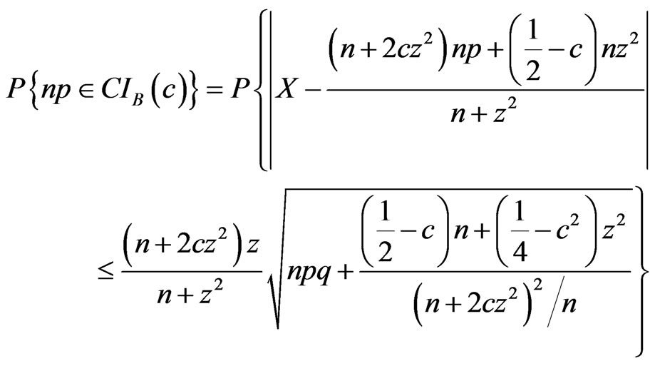
2) If X~B(n, p), the moved score interval on the mean is defined as
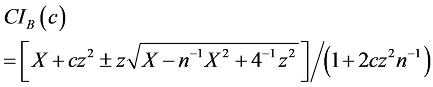
and its coverage probability is equal to
3) If X~NB(r,p), the moved score interval on the Mean is defined as
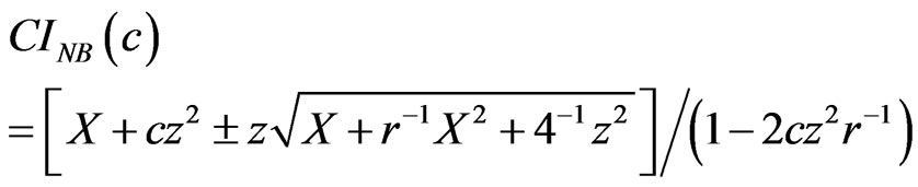
and its coverage probability is equal to

3. Moved Score Interval for the Mean of a Poisson Variable
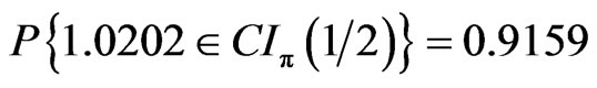
Let X~π (λ),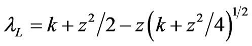 . Set k = 1, 2, 3, 1 – α = 0.95 and z = 1.95996, we have λL = 0.17652, 0.54847, 1.02027 respectively. If λ take values less than λL a little as λ = 0.1765, 0.5484, 1.0202, small coverage probabilities arise.
 .
.
0.8382 is less than the nominal level 0.95 markedly. In the same way, 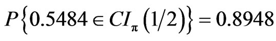 ,
, .
.
Let the mean λ be small near 0, its lower bound of confidence interval should be 0. That is to say, two-sided confidence interval is exactly one-sided interval for the small means. Denote λα* as the upper bound on the mean that two-sided confidence interval can be replaced by one-sided interval, and it could be estimated approximately by P{X ≥ 1 |λα*} = α.
Set
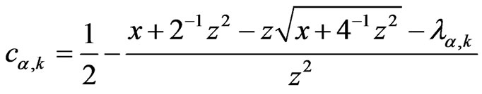
where λα,k is be the real number satisfying P{X ≥ k | λ = λα,k } =1 – α; k = 1,2, ··· ,Kα; Kα is the largest integer such that λα,k ≤ λα*.
Figure 1 shows that most of coverage probabilities of CIπ(0.45) and CIπ(0.44) are not less than the level for λ ≤ λα*. But they seem to be conservative. Numerical computation shows c = 0.46 is almost the best choice on Poisson, binomial and negative binomial variables for general levels 0.90, 0.95, 0.99. In the latter part of this paper would mainly demonstrate advantages of CI(0.46) (see Figure 2).
An important criterion to judge a confidence interval
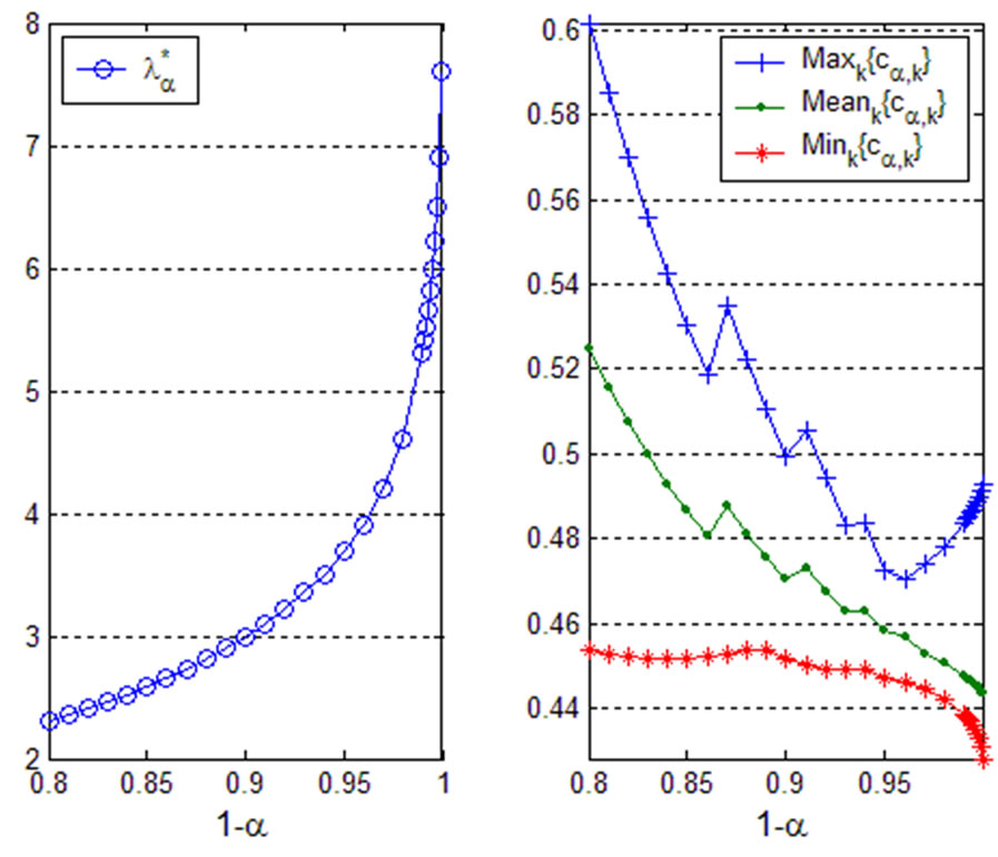
Figure 1. For 1 – α = 0.80,0.81,···,0.99 and 1 – α = 0.991, 00.992,···,0.999, the left panel figures λα* such that P{X ≥ 1 |λα*} = α/2, and the right panel figures the maximum Maxk{cα,k}, the average Mean k{cα,k}, and the minimum Min k{cα,k} for k ≤ Kα from top to bottom curve.
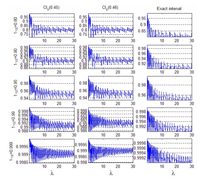
Figure 2. Coverage probabilities of the moved intervals CIπ(0.45) (left panels), CIπ(0.46) (middle panels) and exact interval (right panels) for λ ∈ [0.01,30] on π (λ) with the levels 0.8, 0.90, 0.95, 0.99, 0.999 (from the top to the bottom panels).
is the confidence coefficient, i.e. the infimum of the coverage probability (ICP) of the interval [4]. If ICP < 1 – α, the larger is ICP the better is the interval.
Figure 2 and Table 1 show that CIπ(0.46) and CIπ (0.45) greatly increase ICP and evidently improve the spike characteristic of CIπ(0.5) for small λ. Of course, CIπ(0.46) is more excellent than CIπ(0.45).
Table 2 from [5] lists other eight approximate intervals as the First Normal, with Correction, Bartlett, Mole-
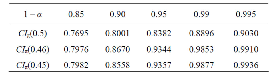
Table 1. The confidence coefficients of CIπ(0.5), CIπ(0.46), CIπ(0.45) on Poisson variable.
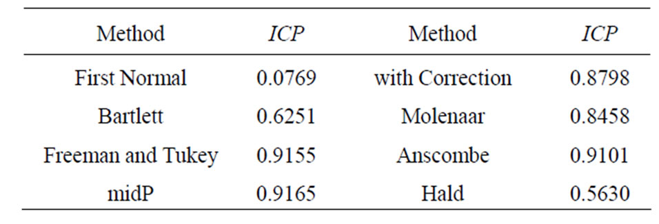
Table 2. The confidence coefficients of some other approximate confidence intervals on Poisson variable when 1 – α = 0.95.
naar, Freeman and Tukey, Anscombe, midP, Hald interval, their ICP are equal to 0.0769, 0.8798, 0.6251, 0.8458, 0.9155, 0.9101, 0.9165, 0.5630 respectively. They are all worse than the moved score interval CIπ(0.46).
For confidence levels 1 – α, Table 3 lists ratios of the confidence probabilities located in intervals 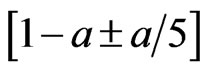 on CIπ(0.5), CIπ(0.46), CIπ(0.45) and the exact interval for λ = 0.001t (= 1,2, ··· , 30000). When 1 – α = 0.85, 0.90, 0.95, 0.99, 0.995, intervals
  = [0.82, 0.88], [0.88, 0.92], [0.94, 0.96], [0.988, 0.992], [0.994, 0.996] respectively. The larger is the ratio, the more is there coverage probabilities close to the level. Table 3 shows that errors between coverage probabilities and levels on the score interval and moved score intervals are analogous to the exact interval, although they do not gurantee all coverage probabilities are not less than levels as the later.
4. Moved Score Intervals for the Means of Binomial Variable and Negative Binomial Variable
Let X~B(n,p ), when p near 0 and 1, π(np) could be as an approximation to B(n,p). So we pay attention to CIB(0.45) and CIB(0.46) also. Agresti and Coull [6], Agresti and Caffo [1] suggested the score interval and the Agresti-Coull interval; Brown et al. [3,7,8] recommended the Agresti-Coull interval, the modified Wilson (score) interval, modified Jeffreys interval and the likelihood ratio interval; Vollset [9] also recommended score methods for its easily computation; Zhou et al. [10] recommended the score interval if there is no available information about p. We believe that the score method is the uppermost approximation on interval estimation of a binomial proportion.
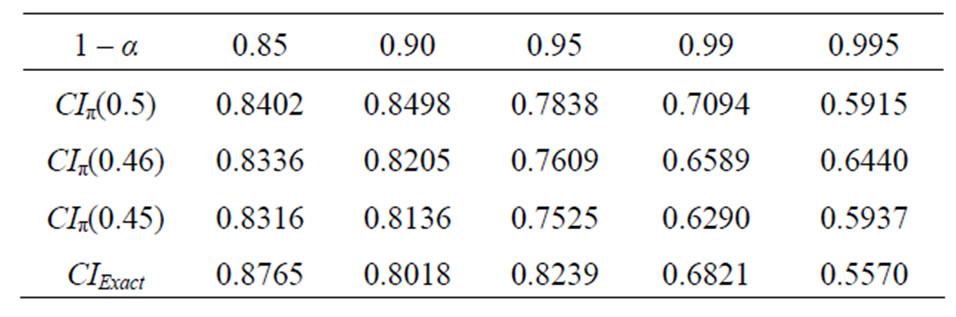
Table 3. Ratios of confidence probabilities of CIπ(0.5), CIπ(0.46), CIπ(0.45) and the exact interval on Poisson variable.
Figure 3 shows that intervals CIB(0.46) and CIB(0.45) improves the spikes of CIB(0.5) obviously. For small p the Agresti-Coull interval behaves too conservative. The Jeffreys interval is a better interval for moderate p, but it has sharp spikes for small p also. Brown et al. [3] suggested revising two specific limits when X = 0, 1, n – 1, or n. Besides, they used one-sided Poisson approximation to binomial distribution to modify CIS with X = 1,2 for n < 50 and X = 3 for n ≥ 50. Numerical computation shows the modified score interval and the modified Jeffreys interval are comparable with moved score intervals CIB(0.46), but the latter method and formula are more simple than the formers. Zhou et al. [10] proposed ZL interval based on logit transformation, but its coverage probabilities are greater than the nominal level when p is close to 0 or 1.
Let X~NB(r,p), when p near 0 and r large, π (rp/q) could be as an approximation to NB(r, p). By numerical computation, we believe CINB(0.45) and CINB(0.46) improve the spikes of CINB(0.5) obviously also. There is
Figure 3 Coverage probabilities of the exact interval (the first row panel), the score interval CIB(0.5) (the second row panel), the moved intervals CIB(0.46) (the third row panel) and CIB(0.45) (the forth row panel),the Agresti-Coull interval CIAC (the fifth row panel) and the Jeffreys interval CIJ (the bottom panel) for B(50, p) with p = 0.001, 0.002,···,0.500 for levels 0.90, 0.95, 0.99 (from the left to the right panels).
fewer people interesting confidence interval on negative binomial variable than binomial variable markedly.
5. Edgeworth Expansion
Brown et al. [3,7,8] suggested utilizing Edgeworth expansion to theoretically analyze the coverage probability of a confidence interval. In general, the intervals for Poisson, binomial and negative binomial variable based on the same method almost have the same Edgeworth expansion (see [8]). So, we only discuss Edgeworth expansion of the moved interval on binomial variable in this section.
Let where
where

Set ,
,  ,
,
 , By lemma 1 in [3], we obtain
Theorem 3 Suppose  is not an integer. Then the coverage probability of CIB(c) satisfies
 where
where
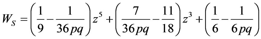
WS is the coefficient of O(n–1) nonoscillating term of the score interval CIB(0.5).
Remark 1. In theorem 3, the first O(n–1) term is nonoscillating and would produce systematic bias without it. So it is a key term. We called its coefficient by coefficient of O(n–1) nonoscillating term. Meanings of other terms in theorem 3 are explained in detail in [3,8].
By theorem 3, the coefficient of O(n–1) nonoscillating term of CI(c) is

Coefficients of O(n–1) nonoscillating terms of the Agresti-Coull interval, the Jeffreys interval and the likelihood ratio interval list as follows (from [8]):
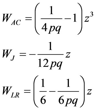
It is easily validated that WAC ≥ WMS(0.46) ≥ WS ≥ WJ ≥ WLR.
See Figure 4. For moderate p, the coefficient of CIB(0.5) is the most close to 0. This ensures the score interval behaves well for moderate p. The moved intrval CIB(0.46) is more conservative than CIB(0.5) a little. The CIAC is too conservative obviously. Coefficients of CIJ and CILR are not larger than –z/3 and –z/2, and too small. Let n = 200, by computation, ratios of coverage probabilities of CIJ not larger than levels 0.90, 0.95 and 0.99 are about 53%, 51% and 54% respectively. In the meanwhile, ratios of CIB(0.46) and CIAC are about 48%, 43%, 40% and 42%, 34%, 28% respectively. Thus, the Jeffreys interval is more stingy than CIB(0.46).

Figure 4. Coefficients of O(n–1) nonoscillating terms of the coverage probabilities of CIAC, CIB(0.46), CIB(0.5), CIJ and CILR (from the top to the bottom curve) with levels 1 – α = 0.80, 0.90, 0.95, 0.99.
Brown et al. [5] showed the ranking expected length of the intervals is CILR, CIJ and CIB(0.5) from the shortest to the longest, provided z > 0.86. Of course their differences are less. On the other hand, the length of interval CIB(0.46) is equal to the score interval for moderate p. Therefore, the expected length of CIB(0.46) is larger than CILR and CIJ a little for z > 0.86.
6. Conclusions and Recommendation
The score interval is concerned all the time by many statisticians for simple formula and good natures. But it has sharp downward spikes for the small mean, since discreteness and skewness cause this problem. Moving the score interval left a little could improve it, though spike phenomena could not be overcome completely.
We recommend the moved score intervals CIπ(0.46), CIB(0.46) and CINB(0.46) respectively for the means of Poisson variable, binomial variable and negative binomial variable as follows

Especially for small Means CI(0.45) is analogous to CI(0.46), but CI(0.45) behaves more conservative than CI(0.46).
7. Acknowledgements
This research is partially supported by Educational Commission of Zhejiang Province of China grant Y2010- 17279.
8. References
[1] P. Kabaila and J. Byrne, “Exact Short Poisson Confidence Intervals,” Canadian Journal of Statistics, Vol. 29, No. 1, 2001, pp. 99-106. doi:10.2307/3316053
[2] A. Agresti and B. Coull, “Approximate Is Better than ‘Exact’ for Interval Estimation of Binomial Proportions,” The American Statistician, Vol. 52, No. 2, 1998, pp. 119 -126. doi:10.2307/2685469
[3] L. D. Brown, T. T. Cai and A. DasGupta, “Interval Estimation intervals for a Binomial Proportion and Asymptotic Expansion,” The Annals of Statistics, Vol. 30, No. 1, 2002, pp. 160-201.
[4] G. Casella and R. L. Berger, “Statistical Inference,” 2nd Edition, Wadsworth, West Yorkshire, 2002.
[5] J. Byrne and P. Kabaila, “Comparison of Poisson Confidence Intervals,” Communications in Statistics-Theory and Methods, Vol. 34, No. 3, 2005, pp. 545-556. doi:10.1081/STA-200052109
[6] A. Agresti and B. Caffo, “Simple and Effective Confidence Intervals for Proportions and Differences of Proportions Result from Adding Two Successes and Two Failures,” The American Statistician, Vol. 54, No. 4, 2000, pp. 280-288. doi:10.2307/2685779
[7] L. D. Brown, T. T. Cai and A. DasGupta, “Confidence Intervals for a Binomial Proportion and Asymptotic Expansion,” The Annals of Statistics, Vol. 30, No. 1, 2002, pp. 160-201.
[8] L. D. Brown, T. T. Cai and A. DasGupta, “Interval Estimation in Exponential Families,” Statistica Sinica, Vol. 13, 2003, pp. 19-49.
[9] S. E. Vollset, “Confidence Intervals for a Binomial Proportion,” Statistics in Medicine, Vol. 12, No. 9, 1993, pp. 809-824. doi:10.1002/sim.4780120902
[10] X. H. Zhou, C. M. Li and Z. Yang, “Improving Interval Estimation of Binomial Proportions,” Philosophical Transactions of the Royal Society A, Vol. 366, No. 1874, 2008, pp. 2405-2418. doi:10.1098/rsta.2008.0037