Open Journal of Geology
Vol.04 No.12(2014), Article ID:52670,17 pages
10.4236/ojg.2014.412048
Shallow-Water Origin of a Devonian Black Shale, Cleveland Shale Member (Ohio Shale), Northeastern Ohio, USA
Saeed Alshahrani1,2, James E. Evans1*
1Department of Geology, Bowling Green State University, Bowling Green, OH, USA
2EXPEC Advanced Research Center, Saudi ARAMCO, Dhahran, Saudi Arabia
Email: *evansje@bgsu.edu
Copyright © 2014 by authors and Scientific Research Publishing Inc.
This work is licensed under the Creative Commons Attribution International License (CC BY).
http://creativecommons.org/licenses/by/4.0/


Received 21 October 2014; revised 18 November 2014; accepted 15 December 2014
ABSTRACT
Black shales are usually interpreted to require anoxic bottom waters and deeper water sedimentation. There has long been a debate about whether the Devonian Cleveland Shale Member of the Ohio Shale (CSM) was deposited in shallow- or deep-water depositional environments. This study looked at the CSM at 3 stratigraphic sections and 5 well cores in northeastern Ohio. The CSM mostly consists of sapropelite (interbedded carbonaceous black mudstones and gray calcareous claystones). The black and gray “shales” are rhythmically bedded at micro- (<1 cm thick), meso- (<10 cm thick) and macro-scales (10s of cm thick) and represent changes in organic matter content (ranging from 7% - 20% TOC). Three types of event layers are interbedded with the mudrocks: 1) tempestites, 2) proximal turbidites, and 3) hyperpycnites. Individual tempestites and turbidites are laterally continuous ≥35 km, while hyperpycnites are too thin (<1 cm) to trace laterally. Tempestites consist of hummocky stratified sandstones with groove casts and escape burrows overlain by planar laminated sandstones with wave ripples at the top. Tempestites average 13 cm thick, but can be amalgamated up to 45 cm thick, and are more common in the lower half of the unit. Turbidites are incomplete Bouma sequences that average 6 cm thick, show evidence of combined flow (“wave-modified turbidites”), and are more common toward the top of the unit. Hyperpycnites (density underflows from river discharge) consist of inverse-to-normal graded sandy or silty microlaminae that have been studied primarily by using petrography and SEM. Condensed sections in the CSM are probable firmgrounds with carbonate concretions, and indicate intervals of low sedimentation rates. The evidence shows that the CSM depositional environment was receiving siliciclastics from the northeast (e.g., Catskill delta), and that the coarser-grained clastic sediment was primarily transported as density underflows (turbidites and hyperpycnites). However, significant storm deposits (tempestites) within the CSM indicate erosion and redeposition occurred on a muddy clastic marine shelf at paleo-water depths less than storm-weather wave base (probably ≤50 m depth).
Keywords:
Black Shales, Tempestites, Hyperpycnites, Devonian, Appalachian Basin, Catskill Delta

1. Introduction
Black shales are defined as mudrocks that have >3% organic carbon, a mole fraction of Fe2+ > 0.8 (mole fraction
 ), and a Munsell Color Value of N1 [1] . Black shales have long been studied as im-
portant petroleum source rocks in conventional petroleum systems [2] . The Devonian black shales in the Appalachian basin (eastern North America) became major targets for conventional oil and natural gas resources starting in the early 1900s [3] , and the Lower Paleozoic total petroleum system including these Devonian black shales had produced about 600 million barrels of oil equivalent (MBBOE) and over 1.5 trillion ft3 (tcf) of natural gas by the 1990s [4] . More recently, the black shales have been recognized as unconventional reservoirs (subject to hydrofracturing) with immense potential, for example the middle Devonian Marcellus Shale is estimated to hold 1307 tcf of recoverable natural gas [5] .
As organic-rich deposits, black shales are known to form in a wide range of environments and geographical settings. Traditionally, the major controls on black shale accumulation were considered to be: the availability of abundant organic matter, types of organic matter, water chemistry, and preservation of organic matter both in the water column and in the sediments (facilitated by rapid deposition and oxygen-deficient conditions) [6] . Of these, the rate of production of organic matter has been considered most critical because decomposition of organic matter consumes available oxygen, and this oxygen deficiency aids in the preservation of organic matter in the water column and sediments [7] . Thus, thick sequences of black shales have been explained using: 1) restricted circulation models where organic matter deposition consumed dissolved oxygen from bottom waters, leading to the reduction of sulfate and production of hydrogen sulfide; 2) open ocean models where organic matter produced in the photic zone was largely recycled, producing an oxygen-minimum zone in the underlying water column which facilitated preservation of a portion of the sedimentary organic matter falling to the sediment interface; and 3) continental shelf models where there was limited recycling of organic matter that was produced in the photic zone (compared to the other two models) because of shorter water residence times prior to settling to the sea floor [6] [7] .
These views have been challenged recently, based on advances in oceanography and biogeochemistry. The more recent view is that relatively few black shales formed under pervasive anoxic bottom water conditions; that the mechanism of water stratification was transient (seasonal or annual thermoclines that formed and deteriorated); and that local suboxic-anoxic conditions in the sediments may have been driven by re-mineralization of bio-limiting nutrients, creating a “euthrophication pump” mechanism in the sediments [8] . This approach treats sedimentation, primary production, and microbial metabolism as interdependent variables [8] . In addition, there is a recognition of the role of sea-level change, for example (in distal parts of the basin), sea-level rise causes sediment starvation, organic carbon concentration in sediments, decreased effectiveness of seasonal mixing, and thus increases the build-up of re-mineralized nutrients. In contrast, sea-level fall results in increased clastic sediment input in distal parts of the basin, dilutes the sediment organic carbon content, causes increased effectiveness of seasonal mixing, and thus decreases the build-up of re-mineralized nutrients in the sediments [8] [9] .
The purpose of this paper is to use sedimentological evidence (facies analysis and microfacies analysis) to resolve the depositional environment of organic-rich black shale from the Late Devonian Cleveland Shale Member (CSM) of the Ohio Shale. The unit contains up to 32% organic carbon [10] in addition to high concentrations of uranium and heavy metals [11] . The organic matter in the CSM is primarily terrigenous plant material including plant macrofossils and abundant spores [12] , but also conodonts and Devonian fish fossils, including at least 22 taxa of arthrodire fish fossils [12] [13] . The sediments are fine-grained and there is a virtual absence of benthic fossils in the black shales [10] . This combination of characteristics caused some earlier researchers to suggest deepwater (≥200 m) conditions with a stratified water column [12] [14] , while others argued for shallow water (≤100 m) euxinic environments that migrated westward as a result of shoreline progradation (“Catskill delta” facies) during the Acadian orogeny [15] . It has been pointed out that neither hypothesis is likely because, on the one hand, it is improbable that the epicontinental sea that covered eastern North America were sufficiently deep for permanent water stratification; and on the other hand, it is also improbable that a shallow water sea could have existed over such a large area and maintained quiet, undisturbed bottom water conditions [10] . An alternative explanation, based on paleoclimatic and tectonic setting, is given in the next section, but it does not specifically address the controversy about water depth.
2. Background
The Ohio Shale was one of the widespread, middle-to-late Devonian organic-rich shales (including the correlative Antrim Shale in Michigan and the Chattanooga Shale in Kentucky and Tennessee) found in the Appalachian basin in eastern North America (Figure 1) [16] [17] . The Ohio Shale is a fissile, dark gray-black, organic-rich shale with minor amounts of siltstone and sandstone. The unit outcrops across central Ohio and along the Ohio River and the coast of Lake Erie, and underlies all of eastern Ohio. The Ohio Shale is an eastward-thickening wedge that ranges from about 10 - 550 m thick, dipping and thickening eastward into the central axis of the Appalachian basin [18] . The Ohio Shale is subdivided into three members; in ascending order these are the Huron Shale Member, Chagrin Shale Member, and Cleveland Shale Member (Figure 1). The Huron Shale Member consists of fissile, black, organic-rich shales with a mean thickness of 125 m. The unit is noted for large (≥2.5 m diameter) carbonate concretions that formed around fossil fish remains [10] [18] . The Huron Shale Member is virtually identical to the Cleveland Shale Member, and the two can only be reliably distinguished if the intervening Chagrin Shale Member is present [11] . The Chagrin Shale Member consists of fossiliferous gray shales that form an eastward-thickening wedge ranging from 0 - 400 m thick in northern Ohio. The unit contains small ironstone concretions built around crustacean, brachiopod, bivalve, cephalopod, conulariid, crinoid, and fish fossils [18] . The Chagrin Shale Member has been interpreted as a clastic wedge related to progradation of the Catskill delta complex from further east. Because of the benthic fossil content, the unit has been interpreted to represent an interruption of anoxic bottom water conditions of the underlying Huron Shale Member and overlying Cleveland Shale Member [15] .
The Cleveland Shale Member (CSM) is another fissile, black, organic-rich shale that is typically 6 - 18 m thick in the study area, and thins both east and west from the study area [19] . The inorganic constituents are primarily quartz, illite, chlorite, and pyrite [15] . The organic constituents are primarily disseminated terrestrial

Figure 1. Correlation diagram for the middle and late Devonian units in the Appalachian basin. The Cleveland Shale Member is the uppermost unit in the Ohio Shale.
organic matter [11] [12] . The unit has distinctive cone-in-cone sedimentary structures in places [11] , and at least three zones of discoid or flattened carbonate concretions in the study area [18] . It is generally recognized that the lower part of the CSM is transitional from the underlying Chagrin Shale Member, with gray shales and siltstones interbedded with fissile black shale, interpreted by some as siltstone turbidites and basinal deposits [19] . The upper part of the unit is mostly black shale, and in places the upper contact of the CSM with the Bedford Shale-Berea Sandstone delta facies shows evidence for load structures and fluid escape structures [19] .
Overall, the region of Middle to Late Devonian black shale deposition was located west of the Acadian tectonic highlands, in a location south of the Late Devonian paleo-equator (Figure 2) [17] . According to one model [17] , the rise of the Acadian tectonic highlands created an orographic barrier to the circulation of the trade winds, preventing moisture from reaching the western side. This model postulates that the decreased rainfall and runoff resulting from an orographic rain shadow effect prevented large volumes of clastic sediment from reaching the Appalachian basin and diluting the organic matter that was generated by primary productivity in the upper portion of the water column. Consequently, high concentrations of organic matter accumulated in the sediment, and lack of an overturning mechanism caused bottom waters and sediments to become oxygen depleted [17] . However, there were also clearly times that active tectonism resulted in the westward progradation of the Catskill delta sequence into the study area, explaining clastic-dominated sequences [10] [17] . In addition, the Appalachian basin was a foreland basin affected by flexure and isostasy [20] , highlighting the possible importance of sea level effects on accumulation of sedimentary organic matter in these black shales [8] [9] .

Figure 2. Paleogeographic reconstruction of North America during the middle and late Devonian. The study area is located in northeastern Ohio, in the Appalachian basin (from [17] ).
3. Material and Methods
3.1. Outcrop Data
After reconnaissance, three sites were selected for measured sections (Figure 3). The stratigraphic section at site 1 (Bay Village, Ohio) is 17 m thick and extends laterally about 330 m (Figure 4). The stratigraphic section at

Figure 3. Location map for northeastern Ohio showing the location of three outcrops (solid squares) and five wells (circles) as well as cities (named). Inset map shows study area location within the State of Ohio (arrow).

Figure 4. Typical outcrop appearance of the Cleveland Shale Member on the coast of Lake Erie. Note the continuity of bedding and event deposits (tempestites, turbidites, and hyperpycnites) interbedded with the shale.
site 2 (Bedford, Ohio), located in the Cuyahoga Valley National Park, is 16 m thick and extends laterals for about 500 m. The stratigraphic section at site 3 (Brooklyn Heights Village Park, Ohio) is 15 m thick and extends laterally for about 450 m. The locations were determined using Garmin GPS (±3 m accuracy). At each location, the stratigraphic section was described in detail, including lithology, composition, texture, and sedimentary structures [21] . Color was determined using a Munsell Color Chart [22] . Outcrop photomosaics were evaluated for stratigraphic architecture. Field work was augmented by 143 collected samples. A total of 68 samples were used to make thin sections for microfacies analysis, and 12 samples were used for SEM/EDAX analysis. Other samples were used for descriptions of sedimentary structures and trace fossils. In addition, a total of 56 paleocurrent measurements were collected using a Brunton compass, and evaluated using standard statistical methods [23] .
3.2. Well Data
After evaluating the inventory of available well data, five wells in northeastern Ohio were selected (Figure 3). The basis of selection was: availability of drill core and geophysical logs from each well, and the presence of the CSM in the section. The cores are stored in the Ohio Geological Survey, H.R. Collins Core Laboratory, in Alum Creek State Park, Ohio. Details about the well locations, drilling history, core length, and core material conditions are given elsewhere [21] . In these five wells, the CSM ranged from 3.3 to 19.5 m thick. Cores were cleaned, photographed, and described using a binocular microscope. A total of 18 samples were collected to make thin sections for microfacies analysis and for SEM/EDAX analysis.
For each well, the available geophysical logs included the gamma-ray log, resistivity log, density log, and caliper log. The details about the geophysical logs and methods of analysis are given elsewhere [21] . The geophysical log pattern for the CSM is distinctive, with a notably higher gamma-ray signature, lower bulk density, and higher resistivity than either the underlying Chagrin Shale Member of the Ohio Shale, or the overlying Bedford Shale (Figure 5). All of these properties are consistent with the higher organic content of the CSM, in

Figure 5. Geophysical log signature for the Cleveland Shale Member, showing high gamma-ray log (GR), low bulk density (D), and high resistivity (R). The caliper log (C) is also shown.
comparison to the underlying and overlying units. The individual well cores could be correlated to their respective geophysical logs, both in overall thickness and such that contacts were about ±0.1 m matches [21] . At a finer scale, sandier intervals (interbedded with the shales) in well cores correspond to lower gamma-ray values, higher bulk densities, and lower resistivity values on the respective geophysical logs [21] .
3.3. Laboratory Analyses
Thin sections were prepared using standard techniques. Using the petrographic microscope at 25× and 40×, point counts were conducted on sandstone samples using the Gazzi-Dickinson method [24] with n > 300 counts per slide. Many core samples were chips too small for standard thin sections, and these were examined as grain mounts using the Leica MZ binocular microscope at 12.5× magnification. SEM samples were prepared using standard techniques [25] , sputter coated with gold-palladium, and examined using a Hitachi model S-2700 Scanning Electron Microscope, with an LaB6 filament, acceleration voltage of 20 kV, beam current (spot size) of 10 A, and working distance of 8 - 12 mm. Elemental determinations used an EDAX SW 9100-60 energy dispersive spectrometer, with a bombardment time of 100 seconds, beam intensity of 20 kV, and sample tilt of 200. Semi-quantitative EDAX analyses were performed using a standard method [26] .
4. Results
4.1. Lithology
Sandstones in the CSM are very fine- to fine-grained, poorly to moderately sorted, sub-angular to subrounded, quartz arenites or quartz wackes (QFL ratio is 92:7:1) [21] . Interbedded sandstones in the CSM represent about 11.4% of the total thickness of the unit. The sandstones contain a variety of primary sedimentary structures including massive bedding, hummocky stratification, planar lamination, ripple lamination, sole marks, fluid escape structures, load structures, and trace fossils. Both normal and inverse grading can be observed. Most of the lithics are sedimentary rock fragments (chert, shale, or siltstone clasts). Accessory minerals include biotite, muscovite, and chlorite. Cements are typically calcite and/or clay minerals. Black opaque grains in sandstones were discovered to be particulate organic matter using the SEM/EDAX [21] .
Siltstones in the CSM are very fine- to coarse-grained, moderate to well sorted, sub-angular to rounded, calcareous quartz siltstones. In the CSM, interlaminated siltstone and mudstone beds a few mm thick represent about 65% of the unit. The siltstones contain a variety of primary sedimentary structures including planar lamination, massive bedding, and micro-cross lamination. The siltstones exhibit both normal and inverse grading, in some instances as part of fining- or coarsening-upward sequences with sandstone. Burrows in the siltstones can be filled by silt- or mud-sized material.
“Shales” in the CSM include organic-rich mudstone, mudshale, claystone, and clayshale. Petrographic analysis shows that the content averages 3% sand (ranges from 0% - 5%), 37% silt (ranges from 5% - 65%), and 49% clay (ranges from 23% - 70%). Particulate organic matter (including plant debris) averages 10% (ranges from 7% - 20%); however this figure may underestimate the very finely disseminated organic component. SEM/ EDAX analysis shows that the principle clay-sized minerals are quartz, chlorite, mixed-layer clays, and illite, with a low (<1%) kaolinite content, consistent with earlier studies [11] [15] . Mud floccules are not observed, probably due to compaction and diagenesis [21] .
4.2. Lithofacies Analysis
This study recognized 14 lithofacies, each defined as a unique combination of lithology, composition, texture, and sedimentary structures (Table 1). Each lithofacies represents a component of a particular depositional environment, and the groupings (or facies associations) and sequences of lithofacies aid in the recognition of ancient depositional environments. The CSM can be considered a rhythmically bedded sequence of mudrocks (siltstones and “shales”) interbedded with episodic deposits (tempestites, turbidites, and hyperpycnites) and hiatuses or breaks in sedimentation represented by condensed sections. Many of these features are fine-scale and can be difficult to observe in outcrop, but can be easily distinguished in polished core sections or in thin sections.
The sapropelite facies association is typically represented by laminated (lithofacies Ml) or massive (lithofacies Mm) black carbonaceous mudstone interbedded with laminated (lithofacies Cl) or massive (lithofacies Cm) dark gray calcareous claystone or marl. The interbedded character of the unit can be observed at different scales,

Table 1. Lithofacies in the Cleveland Shale Member.
ranging from micro-laminae up to distinctive beds at outcrop scale. Such rhythmically interbedded pelagites have been recognized in the geologic literature as sapropelites [27] . On the macro-scale (≥10s of cm), some intervals are characterized by varying amounts of organic matter, such that more organic-rich layers average 13 cm thick and less organic-rich layers average 17 cm [21] . On the meso-scale (1 - 10 cm), bedding intervals have an outcrop appearance of rhythmically bedded (or “varved”) interbedded organic-rich black mudstones and carbonate-rich gray claystones or marls (Figure 6(A)). The stripped appearance is due to the black mudstones (Munsell Color Index N1) weathering various shades of brown (Munsell Color Index 5YR 4/4 to 10YR 4/2) interbedded with dark gray marls (Munsell Color Index N5) weathering to bluish gray (5B 7/1) or greenish gray (5G 6/1). On the micro-scale (<1 cm), closer examination using a binocular microscope (Figure 6(B)) shows micro-laminae within the sapropelite or marl intervals. Note that the textural difference between the mudstones and claystones is the presence of fine-grained particulate organic matter in the mudstones. On a micro-scale, there appears to be repeated packages of thinning-upwards, sapropelite micro-laminae within one marl layer (Figure 6(B)). SEM analysis of the clay minerals reveals both the sapropelite and marl consist of chlorite (Figure 6(C)), mixed-layer clay (Figure 6(D)) and illite (Figure 6(E)), with varying amounts of organic matter and carbonate. In summary, the nature of these “varves” appears to be alternating organic-rich sediment and carbonate-rich sediment.
The hemipelagite facies association consists of intervals of thinly interbedded quartz siltstone and sapropelite (lithofacies SSMl). An example is shown in Figure 6(F). These are interpreted as a variation of the sapropelite facies association that includes frequent episodic introduction of siliciclastic material (possibly as distal turbidites or distal hyperpycnites). Such deposits are classified in the geologic literature as hemipelagites [28] , and represent basinal environments influenced by adjacent sources of terrigenous sediment. In the CSM, hemipelagite intervals have a mean thickness of 19 cm.
The tempestite facies association consists of hummocky stratified very fine- to fine-grained sandstones (lithofacies Sh) overlain by planar laminated sandstone (lithofacies Sl), and ripple laminated sandstone (lithofacies

Figure 6. Sapropelite facies association in the Cleveland Shale Member. (A) Field photograph showing meso-scale (1 - 10 cm thick) alternating black (weathers brown) carbonaceous mudstones and gray (weathers blue-gray) calcareous claystones, or “varves”. Scale bar 15 cm. (B) Polished core section showing micro-scale (<1 cm thick) interbedded carbonaceous mudstones and calcareous claystones, within the thicker (meso-scale) sapropelite or marl beds. Note thinning-upward bedding trend of carbonaceous mudstone laminae within marl bed. Scale bar 1 cm. (C)-(E) SEM images of chlorite (C), mixed layer clays (D), and illite (E), with scale bars shown. Identifications were partly based on matching EDAX profiles, given in [21] . (F)-(G) Photomicrograph of hemipelagite (interbedded marl and sapropelite) with crossed polars (F) and plane-polarized light (G).
Sr), often terminating in wave ripplemarks (Figure 7(A)). The base of the sequence is typically erosional (Figure 7(B)), and may demonstrate groovecasts (Figure 7(C)) or flutecasts. In other cases the base of tempestites includes casts of tracks, trails, and shallow burrows made by benthic organisms (including Neonereites and Planolites) on the upper surface of the underlying mudrocks (Figure 7(D)). Some of the tempestites are amalgamated (i.e., one tempestite directly overlies another tempestite). This amalgamation forms when the upper part

Figure 7. Tempestites (storm deposits) in the Cleveland Shale Member. (A) Field photograph of low-relief erosional base overlain by hummocky stratified sandstone and wave ripples (pencil = 14 cm). (B) Polished core section showing small-scale tempestite with erosional scour at the base overlain by hummocky stratified sandstone and wave ripples. Scale bar 1 cm. (C) Field photograph of groove casts (arrow) at the base of a tempestite (hummocky stratified sandstone, planar laminated sandstone and wave rippled sandstone). Scale bar 15 cm. (D) Field photograph of casts of Planolites burrows (arrow) on sole of a tempestite bed. Scale bar 15 cm.
of the previous tempestite was eroded by the storm event that emplaced the second tempestite. The tempestites in the CSM have a mean thickness of about 13 cm (range 4 - 21 cm), but amalgamated sequences can be up to 40 cm thick. These sequences of deposits are interpreted as storm deposits, in other words they are the results of combined flow due to erosion, re-suspension, and deposition by high energy waves in a shallow water environment [29] [30] .
The turbidite facies assemblagevconsists of massive normally graded sandstone (lithofacies Smg), planar laminated sandstone (lithofacies Sl), ripple-laminated sandstone (lithofacies Sr), laminated siltstone (lithofacies SSl) and laminated or massive mudrocks (lithofacies Ml or Mm). The base of each sequence is erosional with scour marks and tool marks (Figure 8(A)). The deposits can be recognized as turbidites, comprised of the characteristic Bouma sequences (divisions A-E), which can be abbreviated as Tabcde. In the CSM, most turbidites are incomplete Bouma sequences with the observed most common variants being: Tab, Tabc, Tbc, Tae, or Tbe (Figure 8(B)). The average thickness of turbidites in the CSM is about 6 cm, but these range upward to 40 cm thick. The upper portion of individual turbidites often includes combined-flow ripples (Figure 8(C)), and also may include fluid escape structures. Similar deposits have been called “wave-modified turbidites” [31] . Previous studies have interpreted wave-modified turbidites are similar to those observed in the CSM as hyperpycnal-flow generated, prodelta turbidites [32] .
The hyperpycnite facies assemblage consists of thin, laterally discontinuous, sandstone or siltstone in thick sequences of shale (Figure 9(A)). In the field, weathering can make it difficult to distinguish hyperpycnites from distal turbidites or distal tempestites. However, when examined using the microscope, the characteristic properties of hyperpycnites [33] can be readily recognized. Two types of hyperpycnites are present in the CSM. Sandy hyperpycnites consist of massive, inverse- (lithofacies Smi) to normally- (lithofacies Smg) graded sandstones, while silty hyperpycnites consist of massive, inverse- (lithofacies SSmi) to normally- (lithofacies SSmg) graded siltstone. Sandy hyperpycnites may include a middle phase of planar laminated sandstone (lithofacies Sl) or ripple laminated sandstone (lithofacies Sr) (Figure 9(A)). The basal contacts are typically non-erosive. The upper and lower contacts typically grade into the “background” sapropelite deposits (Figure 9(B)). The presence of features such as escape burrows (Figure 9(B)) and fluid escape structures demonstrates that these are event layers. Most of the hyperpycnites in the CSM are <1 cm thick, but in measured sections the mean thickness was

Figure 8. Turbidite facies association in the Cleveland Shale Member. (A) Field photograph of turbidite with an erosional base overlain by fining-upward sandstone (Ta) and planar laminated sandstone (Tb) (scale bar 15 cm). (B) Polished core section showing amalgamated turbidites with wave ripples (wave-modified turbidites) (scale bar 1 cm). (C) Polished core section showing interbedded wave-modified turbidites and hyperpycnites (scale bar 1 cm).

Figure 9. Hyperpycnites (flood deposits) in the Cleveland Shale Member. (A) Field photographs showing typical outcrop appearance of thin, sandy hyperpycnites interbedded with shales. Pen = 14 cm. (B) Polished core section showing series of hyperpycnites, each with an initial coarsening- upward (C-U) base culminating in current ripples, and overlain by a fining-upward (F-U) upper section. Note the escape burrow in one hyperpycnite. Scale bar 1 cm.
found to be 1.7 cm, this value being artificially larger because of the difficulty of recognizing and measuring the thinner hyperpycnites in the field.
The condensed section facies assemblage consists of discrete layers of massive (lithofacies Mm) and concretionary (lithofacies Mmc) calcareous mudstones, often extensively burrowed. The concretions are vertically-flattened, discoid shapes in cross-section. Laterally, they range from individual nucleation sites (round) to irregular shapes caused by a number of coalesced nucleation sites (Figure 10(A)). The trace fossils in these layers are dominated by burrows such as Psilonichnus (Figure 10(B)), which contrast to the more typical tracks and bedding-parallel structures observed elsewhere (e.g., Figure 7(D)). The combination of carbonate cement, concretions, and vertical burrows suggests that layers were firmgrounds [34] , representing sediment packages that

Figure 10. Condensed sections in the Cleveland Shale Member. (A) Small examples of carbonate concretions, which tend to be found in layers, may be coalesced from several initially round growth centers, and are often flattened (scale bar 5 cm). (B) Psilonichnus burrows on the upper bedding surface of a carbonate-rich mudstone interbedded with other mudstones, representing a possible firmground (scale bar 3 cm).
became semi-consolidated due to low deposition rates or a hiatus.
4.3. Event Layer Correlations
Individual tempestites, and especially intervals of amalgamated tempestites, can be correlated over a distance of ≥35 km between the three outcrops (Figure 11). With less certainty, notable sandier intervals (comprised of a number of beds of tempestites and/or turbidites) can be correlated in the subsurface over a distance of up to 75 km [21] . Tempestites are the deposits of major storms in shallow-water environments [30] . These event deposits form in water depths above storm-weather wave base, but because of subsequent re-working by fair-weather waves, the deposits might not be preserved at water depths above fair-weather wave base [35] . In other words, tempestites are most commonly preserved in the offshore transition zone, at water depths typically ranging between 50 - 100 m deep (the boundary between the offshore zone and the offshore transition zone) to 10 - 30 m deep (the boundary between the offshore transition zone and the lower shoreface zone) [36] . In addition, some of the tempestites in the CSM show significantly erosive bases, the presence of intraclasts, and amalgamation. These “proximal tempestites” would be expected to form at the shallow range of water depths given above (i.e., near the boundary between the offshore transition zone and the lower shoreface zone) [37] . In summary, tempestites are shallow water storm deposits, and the ability to correlate individual sandy storm deposits over distances of 10s of km, in an overall muddy sequence, suggests an extensive, shallow water, muddy shelf depositional environment that was affected by episodic major storms.
4.4. Paleocurrent Data
Paleocurrent data using groove casts at site 1 are shown in Figure 12. Groove casts are bidirectional indicators, but the data are interpreted to show paleoflow to the west-southwest based on facies relationships, thickness trends, and earlier studies [19] . Paleogeographic relationships [10] suggest the major source of siliciclastic sediment was to the east-northeast, or in other words the Catskill delta facies (Figure 2).
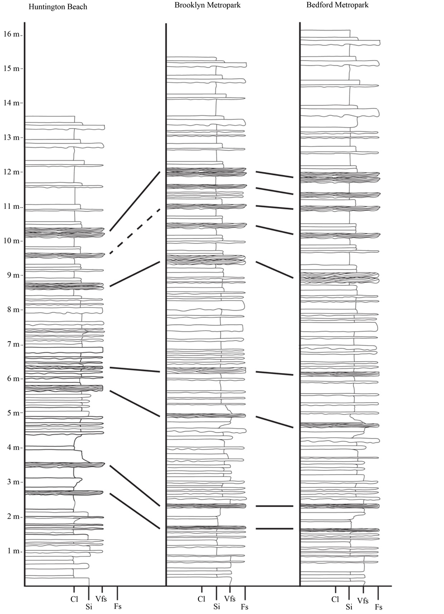
Figure 11. Correlation of tempestites from Huntington Beach to Brooklyn Metropark (23 km) to Bedford Metropark (12 km). Grain size scale abbreviations Cl = shale, Si = siltstone, Vfs = very fine-grained sandstone, and Fs = fine-grained sandstone.

Figure 12. Paleocurrent rose diagram for the Cleveland Shale Member, based upon bi- directional indicators such as groove casts. See text for discussion.
5. Discussion
5.1. Implications of Sandy and Silty Deposits in the CSM
The coarser-grained siliciclastics (sandstone and siltstone) in the CSM are event deposits: turbidites, tempestites, and hyperpycnites. These show two additional characteristics: 1) the importance of density underflows (turbidites and hyperpycnites) in transporting the coarser-grained siliciclastics into a mud-dominated marine environment, and 2) the importance of wave processes in modifying or re-working those coarser-grained siliciclastics (tempestites and wave-modified turbidites) within the marine mud-dominated environment. Our observations are consistent with recent findings that marine shelf sequences often include marine-mudstone encased, prodelta turbidite complexes [32] . Marine hyperpycnal flows are generated at river mouths during river flood events, where the river suspended sediment plume plunges to the seafloor, and the resulting hyperpycnal flow is capable of erosion, transport of sand and silt into deeper water, and deposition [38] . In the Book Cliffs (Utah), similar deposits in the Cretaceous Mancos Shale are interpreted to have been deposited at paleo-water depths of 10 - 20 m [32] . Density underflows were clearly the dominant process of transporting coarser-grained siliciclastic sediment, for example, one 14-m stratigraphic section contained 24 hyperpycnite event layers and 4 turbidite event layers.
The importance of wave modification or re-working in these deposits cannot be over-stated. Wave modification processes occur at or above storm-weather wavebase, which can be as deep as 100 m in some modern open shelf environments, but was more likely to have been significantly shallower (probably ≤50 m paleo-water depth) in these epicontinental seaway deposits. Further, the presence of proximal tempestites (amalgamated hummocky stratified sandstones) is suggestive of deposition toward the deeper end of the lower shoreface zone (possibly 10 - 30 m paleo-water depth). In addition, the presence of combined ripples in turbidites indicates that the turbidites were also deposited above storm-weather wavebase, and not deposited in basinal (below storm-weather wavebase) conditions.
5.2. Implications of Sapropelites in the CSM
The bulk of the CSM consists of carbonaceous black mudstones and mudshales interbedded with gray calcareous claystones and clayshales. The black and gray “shales” are interbedded on micro- (<1 cm), meso- (1 - 10 cm), and macro- (10s of cm) scales. The shales are also interbedded with wave modified or wave re-worked deposits, and trace fossils (predominantly bedding plane tracks and trails) are relatively common. These characteristics are not consistent with a depositional model requiring permanent water column stratification and anoxic bottom water conditions.
The observed scale differences in bedding patterns suggest multiple variables may be explaining the cyclicity. On a micro-scale (<1 cm thick), the rhythmically bedded black and gray “shales” represent variations in organic matter content. The black mudstones and mudshales contain more silt and particulate organic matter than the more carbonate-rich gray claystones and clayshales (Figure 6(B)). Rhythmic bedding on the micro-scale might, therefore, be attributed to the episodic occurrence of plankton blooms (marls) and intervening episodic flood events that generated hyperpycnal flows, and transported silt and terrigenous particulate organics (sapropelites) to the basin. The evidence would also suggest that any form of density stratification (i.e. formation of a pycnocline) would have been transient, interrupted by water column mixing inherent in wave re-working of the sediment (tempestites and wave modified turbidites). The rate of burial and anoxic conditions in the sediment may have played a key role in organic matter concentration and preservation.
Previous researchers have noted that variations in organic carbon (measured as TOC) and Fe-sulfides (measured as total sulfur or TS) in the CSM correlate to gray-scale density values [39] . The black (high TOC/low TS) layers were found to have large amounts of poorly preserved (i.e., bacterially reworked) organic matter, while the gray (low TOC/high TS) layers were found to contain smaller quantities of well-preserved organic matter of mostly marine algal origin [39] . These observations were interpreted to show that the black mudstones (with a higher silt content) represented lower bulk sedimentation rates, allowing bacterial reworking and concentration of organic matter, while the gray claystones were deposited at higher bulk sedimentation rates, allowing better preservation of organic matter and a greater flux of reactive Fe for precipitation of authigenic Fe-sulfides [39] . It is not clear from reference [39] which scale of cyclicity was evaluated, and these results are more consistent with our observations for meso-scale cyclicity described below.
On the meso-scale (1 - 10 cm thick), the “varves” evident at outcrop scale (Figure 6(A)) are packages of sapropelites-dominated or marl-dominated sediment, both containing the micro-scale rhythmicity described above, but showing greater or lesser importance of the black or gray shale end-members. Climate-induced cycles have been used to explain rhythmic bedding patterns in sapropelites. For example, Cenozoic sapropelites in the Mediterranean Sea area have been explained using wet-dry oscillations caused by precession-induced insolation variations, such that wetter conditions (northern hemisphere summer insolation maxima) favor increased continental run-off, higher nutrient flux to the basin, a reduction in evaporation and lesser bottom water formation [40] [41] .
Finally, on the macro-scale (10s of cm thick) the CSM may be interpreted as showing paleo-water depth variations. Most of the tempestites (and all of the amalgamated tempestites) are found in the middle part of the unit. This can be interpreted to show shallowing upward from the lower part of the unit to the middle part, and then deepening upward from the middle part to the top of the unit [21] . Whether or not such changes in water depth/ accommodation space were due to tectonism, such as isostasy and flexure in this foreland basin setting [42] , or were driven by Late Devonian eustatic sea level rise [43] , is beyond the scope of this paper. It has also been proposed that progressive changes upward in the CSM are a result of Late Devonian seawater chemistry variability [45] .
6. Summary and Conclusion
The Cleveland Shale Member is one of a succession of Middle to Late Devonian black shales of the Appalachian basin in eastern North America. Although some of these shales appear to have been formed in deepwater (basinal) anoxic conditions [43] [44] , the Cleveland Shale Member shows clear evidence for deposition above storm-weather wave base, most likely at ≤50 m paleo-water depth. Further, the presence of hyperpycnites and turbidites indicates coarser-grained siliciclastics were transported from source areas in the northeast of the basin, into the study area as density underflows. The presence of tempestites and wave modified turbidites indicates shallow water deposition affected by wave re-working. The presence of rhythmically bedded sapropelite and marl with cyclicity on micro- (<1 cm thick), meso- (1 - 10 cm thick) and macro- (10 s of cm thick) scales indicates multiple mechanisms controlled organic matter deposition and preservation in the CSM depositional system. These may have included: 1) episodic plankton blooms and/or episodic flood events, and the transient formation and dissipation of the pycnocline; 2) progressive climate change affecting run-off, nutrient loading, and the strength of water column mixing; and 3) longer-term trends due to tectonics (flexure and isostasy in a fore- land basin setting) and/or Late Devonian eustatic sea level change.
Acknowledgements
This study was a portion of a master’s thesis at Bowling Green State University. We wish to thank the Ohio Geological Survey, especially Greg Schumacher, for access to cores at the Horace R. Collins Core Laboratory. We thank Dr. Carol Heckman and Marilyn Cayer for assistance with SEM/EDAX analyses and Dr. Margaret Yacobucci for assistance with fossil and trace fossil identifications. The research was financially supported by the Department of Geology Foundation and the Saudi Arabia Culture Mission.
References
- Potter, P.E., Maynard, J.B. and Pryor, W.A. (1980) Sedimentology of Shale. Springer-Verlag, New York, 310 p. http://dx.doi.org/10.1007/978-1-4612-9981-3
- Tissot, B.P. and Welte, D.H. (1978) Petroleum Formation and Occurrence. Springer-Verlag, Heidelberg, 538 p. http://dx.doi.org/10.1007/978-3-642-96446-6
- Schott, G.L., Overbey Jr., W.K., Hunt, A.E. and Komar, C.A. (1978) Document MERC/SP-77/5. 1st Eastern Gas Shales Symposium, U.S. Department of Energy, Morgantown Energy Research Center, 783 p.
- Ryder, R.T., Swezey, C.S., Crangle, R.D. and Trippi, M.H. (2008) Geologic Cross Section E-E’ through the Appalachian Basin from the Findlay Arch, Wood County, Ohio, to the Valley and Ridge Province, Pendleton County, West Virginia. Scientific Investigations Map 2985, U.S. Geological Survey, 53 p.
- Boyce, M.L. and Carr, T.R. (2009) Lithostratigraphy and Petrophysics of the Devonian Marcellus Interval in West Virginia and Southwestern Pennsylvania. AAPG Search and Discovery, Article ID: 90113.
- Didyk, B., Simoneit, B., Brassell, S. and Englinton, G. (1978) Organic Geochemical Indicators of Paleoenvironmental Conditions of Sedimentation. Nature, 272, 216-222. http://dx.doi.org/10.1038/272216a0
- Tourelot, H. (1979) Black Shale: Its Deposition and Diagenesis. Clays and Clay Minerals, 27, 313-321. http://dx.doi.org/10.1346/CCMN.1979.0270501
- Sageman, B.B., Murphy, A.E., Werne, J.P., Ver Straeten, C.A., Hollander, D.J. and Lyons, T.W. (2003) A Tale of Shales: The Relative Roles of Production, Decomposition, and Dilution in the Accumulation of Organic-Rich Strata, Middle-Upper Devonian, Appalachian Basin. Chemical Geology, 195, 229-273. http://dx.doi.org/10.1016/S0009-2541(02)00397-2
- Ver Straeten, C.A., Brett, C.E. and Sageman, B.B. (2011) Mudrock Sequence Stratigraphy: A Multi-Proxy (Sedimentological, Paleobiological, and Geochemical) Approach, Devonian Appalachian Basin. Palaeogeography, Palaeoclimatology, Palaeoecology, 304, 54-73. http://dx.doi.org/10.1016/j.palaeo.2010.10.010
- Hansen, M.C. (1999) The Geology of Ohio―The Devonian. Ohio Geology, No. 1, 1-7.
- Hoover, K.V. (1960) Devonian-Mississippian Shale Sequence in Ohio. Ohio Geological Survey, Information Circular No. 27, 154 p.
- Szmuc, E.J. (1970) The Devonian System. In: Banks, P.O. and Feldmann, R.M., Eds., Guide to the Geology of Northeastern Ohio, Northern Ohio Geological Society, Cleveland, 9-21.
- Feldmann, R.M. and Hackathorn, M. (1996) Fossils of Ohio. Ohio Geological Survey, Bulletin 70, 577 p.
- Rich, J.L. (1951) Probable Fondo Origin of Marcellus-Ohio-New Albany-Chattanooga Bituminous Shales. AAPG Bulletin, 35, 2017-2040.
- Nelson, B.W. (1955) Pre-Berea Mineralogy and Stratigraphy. Ph.D. Dissertation, University of Illinois, Champaign- Urbana, 104 p, Unpublished.
- Janssens, A. (1970) Middle Devonian Formations in the Subsurface of Northwestern Ohio. Ohio Geological Survey, Report of Investigations 78, 22 p.
- Ettensohn, F.R. and Barron, L.S. (1981) Depositional Model for the Devonian-Mississippian Black Shales of North America: A Paleoclimatic-Palaeogeographic Approach. In: Roberts, T.G., Ed., Geological Society of America, Cincinnati’81 Field Trip Guidebooks, Vol. 2, American Geological Institute, Falls Church, 344-357.
- Hansen, M.C. (1994) Ohio Shale Concretions. Ohio Geological Survey, GeoFacts, No. 4, 2 p.
- Lewis, T.L. (1988) Late Devonian and Early Mississippian Distal Basin-Margin Sedimentation of Northern Ohio. Ohio Journal of Science, 88, 23-39.
- Pashin, J.C. and Ettensohn, F.R. (1995) Reevaluation of the Bedford-Berea Sequence in Ohio and Adjacent States: Forced Regression in a Foreland Basin. Geological Society of America Special Paper, 298, 1-69.
- Alshahrani, S.S. (2013) Depositional Environment, History, Diagenesis, and Petroleum Geology of the Cleveland Shale Member, Northeastern Ohio. M.S. Thesis, Bowling Green State University, Bowling Green, 180 p, Unpublished.
- Goddard, E.N., Trask, P.D., DeFord, R.K., Rove, O.N., Singewald Jr., J.T. and Overbeck, R.M. (1948) Rock Color Chart. Geological Society of America, Boulder, 16 p.
- Potter, P.E. and Pettijohn, F.J. (1977) Paleocurrents and Basin Analysis. 2nd Edition, Springer-Verlag, New York, 425 p.
- Ingersoll, R.V., Bullard, T.F., Ford, R.L., Grimm, J.P., Pickle, J.D. and Sares, S.W. (1984) The Effect of Grain Size on Detrital Modes: A Test of the Gazzi-Dickinson Point-Counting Method. Journal of Sedimentary Petrology, 54, 103-116.
- Bozzola, J.J. and Russell, L.D. (1999) Electron Microscopy: Principles and Techniques for Biologists. Jones and Bartlett, Boston, 670 p.
- Beaman, D.R. and Isari, J.A. (1972) Electron Beam Microanalysis. ASTM Special Publication No. 506, Chicago, 102- 108.
- Berger, W.H. (1974) Deep-Sea Sedimentation. In: Burk, C.A. and Drake, C.L., Eds., Geology of the Continental Margins, Springer, New York, 213-241. http://dx.doi.org/10.1007/978-3-662-01141-6_16
- Pickering, K.T., Hiscott, R.N. and Hein, F.J. (1989) Deep Marine Environments: Clastic Sedimentation and Tectonics. Unwin Hyman, London, 416 p.
- Dott Jr., R.H. and Bourgeois, J. (1982) Hummocky Stratification: Significance of Its Variable Bedding Sequences. Geological Society of America Bulletin, 93, 663-680. http://dx.doi.org/10.1130/0016-7606(1982)93<663:HSSOIV>2.0.CO;2
- Einsele, G. (2000) Sedimentary Basins: Evolution, Facies, and Sediment Budgets. Springer-Verlag, Heidelberg, 792 p. http://dx.doi.org/10.1007/978-3-662-04029-4
- Myrow, P.M., Fischer, W. and Goodge, J.W. (2002) Wave-Modified Turbidites: Combined-Flow Shoreline and Shelf Deposits, Cambrian, Antarctica. Journal of Sedimentary Research, 72, 641-656. http://dx.doi.org/10.1306/022102720641
- Pattison, S.A.J. (2005) Storm-Influenced Prodelta Turbidite Complex in the Lower Kenilworth Member at Hatch Mesa, Book Cliffs, Utah, U.S.A.: Implications for Shallow Marine Facies Models. Journal of Sedimentary Research, 75, 420- 439. http://dx.doi.org/10.2110/jsr.2005.033
- Mulder, T., Syvitski, J.P.M., Migeon, S., Faugeres, J.C. and Savoye, B. (2003) Marine Hyperpycnal Flows: Initiation, Behavior, and Related Deposits: A review. Marine and Petroleum Geology, 20, 861-882. http://dx.doi.org/10.1016/j.marpetgeo.2003.01.003
- Frey, R.W. and Pemberton, S.G. (1984) Trace Fossil Facies Models. In: Walker, R.G., Ed., Facies Models, 2nd Edition, American Association of Petroleum Geologists, Tulsa, 189-207.
- Leckie, D.A. and Walker, R.G. (1982) Storm- and Tide-Dominated Shorelines in Late Cretaceous Moosebar-Lower Gates Interval―Outcrop Equivalents of Deep Basin Gas Trap in Western Canada. AAPG Bulletin, 66, 138-157.
- Nichols, G. (1999) Sedimentology and Stratigraphy. Blackwell Science Ltd., Oxford, 355 p.
- Walker, R.G. and Plint, A.G. (1992) Wave- and Storm-Dominated Shallow Marine Systems. In: Walker, R.G. and James, N.P., Eds., Facies Models: Response to Sea Level Change, Geological Association of Canada, GeoText 1, Newfoundland, 219-238.
- Mulder, T. and Syvitski, J.P.M. (1995) Turbidity Currents Generated at River Mouths during Exceptional Discharges to the World Oceans. Journal of Geology, 103, 285-299. http://dx.doi.org/10.1086/629747
- Jaminski, J., Algeo, T.J. and Maynard, J.B. (1998) Climatic Origin of Dm-Scale Compositional Cyclicity in the Upper Devonian Cleveland Member of the Ohio Shale (Abstract). Geological Society of America, Abstracts with Programs, 30, 25.
- Nijenhuis, I.A., Schenau, S.J., Van der Weijden, C.H., Hilgen, F.J., Lourens, L.J. and Zachariasse, W.J. (1996) On the Origin of Upper Miocene Sapropelites: A Case Study from the Faneromeni Section, Crete (Greece). Paleoceanography, 11, 633-645. http://dx.doi.org/10.1029/96PA01963
- Vazquez, A., Utrilla, R., Zamarreno, I., Sierro, F.J., Flores, J.A., Frances, G. and Barcena, M.A. (2000) Precession- Related Sapropelites of the Messinian Sorbas Basin (South Spain): Paleoenvironmental Significance. Palaeogeography, Palaeoclimatology, Palaeoecology, 158, 353-370. http://dx.doi.org/10.1016/S0031-0182(00)00058-4
- Ettensohn, F.R. (2012) Generating Devonian-Mississippian Black Shale Repositories in the Appalachian Basin: Refining the Tectonic Models (Abstract). Geological Society of America, Abstracts with Programs, 44, 6.
- Ettensohn, F.R. (2012) Approximating Water Depths during Deposition of the Devonian-Mississippian Black Shales in the Northern Appalachian Basin (Abstract). Geological Society of America, Abstracts with Programs, 44, 6.
- Ver Straeten, C.A. (2012) Marcellus Black Shale Facies: Constraints and Perspectives on Water Depth (Abstract). Geological Society of America, Abstracts with Programs, 44, 6.
- Algeo, T.J. (2004) Can Marine Anoxic Events Draw down the Trace Element Inventory of Seawater? Geology, 32, 1057-1060.
NOTES

*Corresponding author.