Open Journal of Discrete Mathematics
Vol.1 No.2(2011), Article ID:5740,19 pages DOI:10.4236/ojdm.2011.12009
Mean Square Numerical Methods for Initial Value Random Differential Equations
1 Engineering Mathematics Department, Faculty of Engineering, Cairo University, Giza, Egypt
2 Mathematic Department, Faculty of Science, Mansoura University, Mansoura, Egypt
E-mail: *magdyeltawil@yahoo.com, m_stat2000@yahoo.com
Received April 1, 2011; revised April 30, 2011; accepted May 9, 2011
Keywords: Random Differential Equations, Mean Square Sense, second random variable, Initial Value Problems, Random Euler Method, Random Runge Kutta-2 Method
Abstract
In this paper, the random Euler and random Runge-Kutta of the second order methods are used in solving random differential initial value problems of first order. The conditions of the mean square convergence of the numerical solutions are studied. The statistical properties of the numerical solutions are computed through numerical case studies.
1. Introduction
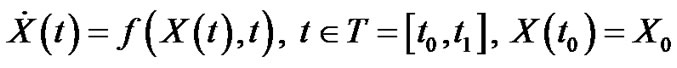
Random differential equations (RDE) are defined as differential equations involving random inputs. In recent years, increasing interest in the numerical solution of (RDE) has led to the progressive development of several numerical methods. This paper is interested in studying the following random differential initial value problem (RIVP) of the form:
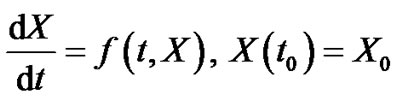 (1.1)
(1.1)
Randomness may exist in the initial value or in the differential operator or both. In [1,2], the authors discussed the general order conditions and a global convergence proof is given for stochastic Runge-Kutta methods applied to stochastic ordinary differential equations (SODEs) of Stratonovich type. In [3,4], the authors discussed the random Euler method and the conditions for the mean square convergence of this problem. In [5], the authors considered a very simple adaptive algorithm based on controlling only the drift component of a time step. Platen, E. [6] discussed discrete time strong and weak approximation methods that are suitable for different applications. Other numerical methods are discussed in [7-12].
In this paper the random Euler and random RungeKutta of the second order methods are used to obtain an approximate solution for equation (1.1). This paper is organized as follows. In Section 2, some important preliminaries are discussed. In Section 3, the existence and uniqueness of the solution of random differential initial value problem is discussed and the convergence of random Euler and random Runge-Kutta of the second order methods is discussed. In Section 4, the statistical properties for the exact and numerical solutions are studied. Section 5 presents the solution of some numerical examples of first order random differential equations using random Euler and random Runge-Kutta of the second order methods showing the convergence of the numerical solutions to the exact ones (if possible). The general conclusions are presented in the end section.
2. Preliminaries
2.1. Mean Square Calculus [13]
Definition1. Let us consider the properties of a class of real r.v.’s  whose second moments,
  are finite. In this case, they are called“second order random variables”, (2.r.v’s).
Definition 2. The linear vector space of second order random variables with inner product, norm and distance, is called an  -space.
A s.p.  is called a “second order stochastic process” (2.s.p) if for
 , the r.v’s
  are elements of
  -space.
A second order s.p.  is characterized by
 ,
, .
.
2.1.1. The Convergence in Mean Square
A sequence of r.v’s  converges in mean square (m.s) to a random variable
if  i.e.
i.e.  or
or
where lim is the limit in mean square sense.
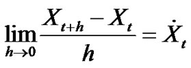
2.1.2. Mean-Square Differentiability
The random process  is mean-square differentiable at t if
  exists, and is denoted by
3. Random Initial Value Problem (RIVP)
3.1. Existence and Uniqueness
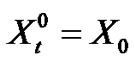
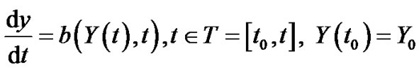
Let us have the random initial value problem
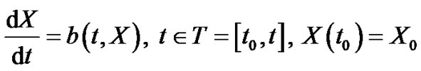 (3.1)
(3.1)
where  is second order random process. This equation is equivalent to integral equation
 (3.2)
(3.2)
Theorem (3.1.1)
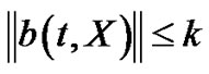
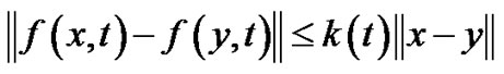
If we have the random initial value problem (3.1) and suppose the right-hand side function  is continuous and satisfies a mean square (m.s) Lipschitz condition in its second argument:
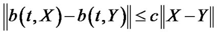 (3.3)
(3.3)
where C is a constant or
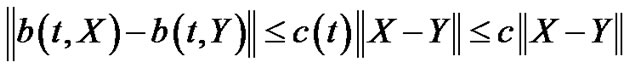 (3.4)
(3.4)
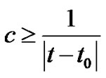
where c(t) is a continuous function {because in every finite interval c(t) ≤ constant}.
then the solution of equation (3.1) exists and is unique.
The proof
The existence can be proved by using successive approximations. Let
 (3.5)
(3.5)
and for n  1
1
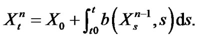 (3.6)
(3.6)
For n  1 we obtain:
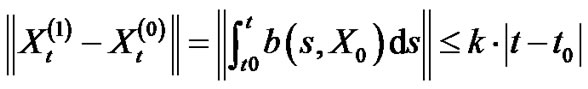
where
 (3.7)
(3.7)
For n > 1 we obtain:
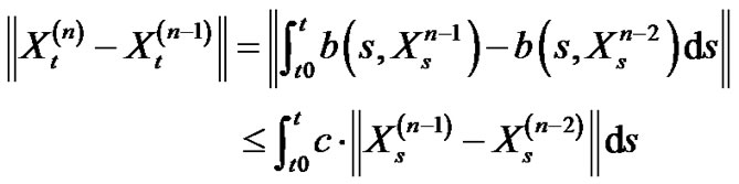 (3.8)
(3.8)
Successively, we can obtain the following:

Hence
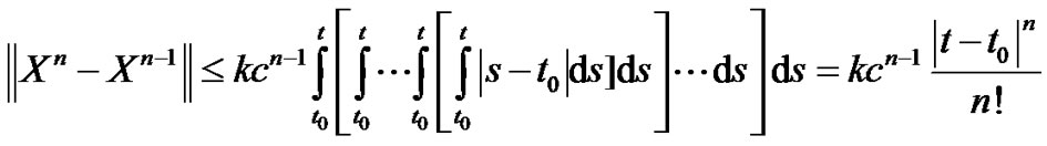 (3.9)
(3.9)
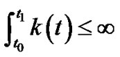
Since:
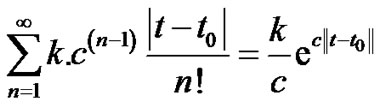 is convergent for finite t,
(3.10)
hence we can have the following
 (3.11)
Accordingly,

Hence:

This yield 
Then 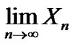 exists. i.e.
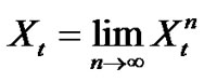 (3.12)
Since  is the general solution of equation (3.6) and
  is the general solution of equation (3.2).
To prove the uniqueness of the solution, let  is a solution of the initial-value problem (3.1), or, which is the same, of the integral equation (3.2), and
  is the solution of
 (3.13)
to prove the uniqueness of the solution we want to prove that
 (3.14)
By subtraction (3.2) and the corresponding integral equation for 
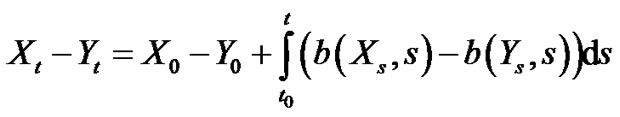
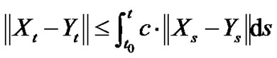
Since 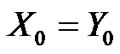 then:
then:
(3.15)
 (3.16)
i.e;
(3.17)
where .
.
(3.18)
From equation (3.17) we have:
 (3.19)
Note that: at  we obtain
  then:
then: 
From (3.19)  must satisfy the following condition:
 (3.20)
which is in contradiction with being an independent free constant, hence the only solution of the integral equation (3.17) is
 (3.21)
Hence  i.e., the solution of equation (3.1) exists and is unique.
3.2. The Convergence of Euler Scheme for Random Differential Equations in (m.s.) Sense
Let us have the random differential equation
 (3.22)
where X0 is a random variable and the unknown  as well as the right-hand side f (X,t) are stochastic processes defined on the same probability space.
Definitions [6,7]
• Let g:  is an m.s. bounded function and let h > 0 then The “m.s. modulus of continuity of g” is the function

• The function g is said to be m.s uniformly continuous in T if:
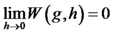
Note that:
(The limit depends on h because g is defined at every t so we can write )
)
In the problem (3.22), we find that the convergence of this problem depends on the right hand side (i.e.  then we want to apply the previous definition on
  hence:
Let  be defined on
  where S is bounded set in
Then we say that f is “randomly bounded uniformly continuous” in S, if

(note that )
)
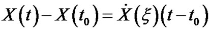
3.2.1. Random Mean Value Theorem for Stochastic Processes
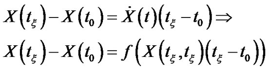
The aim of this section is to establish a relationship between the increment  of a 2-s.p. and its m.s. derivative
  for some
  lying in the interval
  for
for . This result will be used in the next section to prove the convergence of the random Euler method.
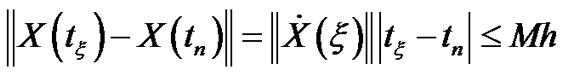
Lemma (3.3.2) [6,7]
Let  is a 2-s.p., m.s. continuous on interval
  . Then, there exists
  such that
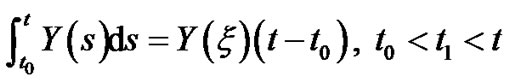 (3.25)
The proof
Since  is m.s. continuous, the integral process
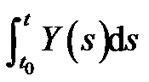 is well defined and the correlation function
 is well defined, is a deterministic continuous function on T × T.
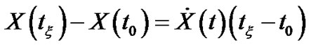
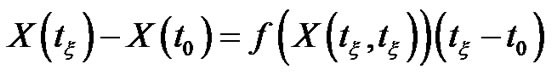
For each fixed r, the function  is continuous and by the classic mean value theorem for integrals, it follows that:
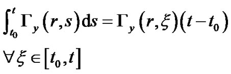 (3.26)
Note that by definition of  expression (3.26) can be written in the form
Since 
We must prove that for the value  satisfying (3.26) one get:
 (3.27)
The proof of (3.27)
As
 (3.28)
and since:
then by substituting in (3.28)
 (3.29)
And since:

then by substituting in (3.28) we have:
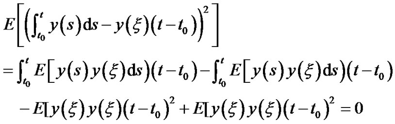
i.e.  we obtain

Theorem (3.3.1) [6,7]
Let  be a m.s. differentiable 2-s.p. in
  and m.s. continuous in
 . Then, there exists
  such that
 ,
,

The proof
The result is a direct consequence of Lemma (3.3.2) applied to the 2-s.p. 

And the integral formula
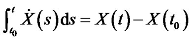 (3.30)
The proof of (3.30)
Let  be a m.s. differentiable on T and let the ordinary function
  be continuous on
  whose partial derivative
 exist If
(3.31)
Then
 (3.32)
Let  in Equations (3.31) and (3.32) we have the useful result that:
If  is m.s. Riemann integrable on T then:

Then we have:

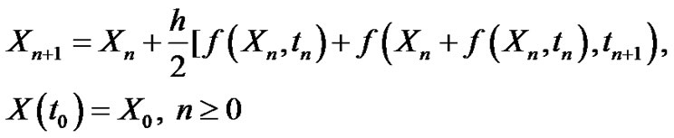
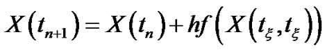
3.2.2. The Convergence of Random Euler Scheme
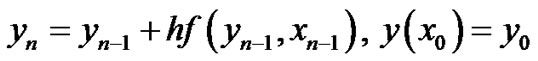
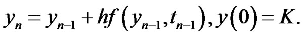
In this section we are interested in the mean square convergence, in the fixed station sense, of the random Euler method defined by
 (3.33)
where  and
and  are 2-r.v.’s ,
  ,
,  and f:
 ,
,  satisfies the following conditions:
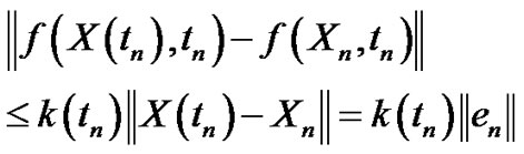
C1:  is randomly bounded uniformly continuousC2:
  satisfies the m.s. Lipschitz condition

where
 (3.34)
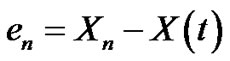
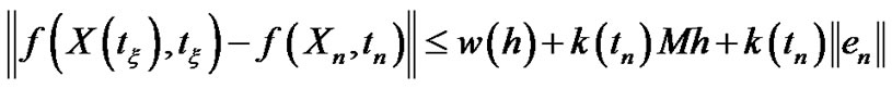
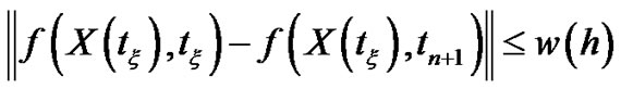
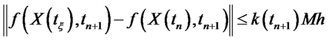
Note that under hypothesis C1 and C2, we are interested in the m.s. convergence to zero of the error
 (3.35)
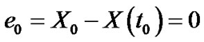
where  is the theoretical solution 2-s.p. of the problem (3.22),
 .
.
Taking into account (3.22), and Theorem (3.3.1), one getsSince from (3.22) we have at  then
then
Note  and we can use
  instead of
  and from Theorem (3.3.1) at
  then we have:
 then
then
Note that we deal with the interval 
 and hence
  was the starting in the problem (3.22) and here
  is the starting and since Euler method deal with solution depend on previous solution and if we have
  instead of
  then we can use
  instead of
 .
.
Then the final form of the problem (3.22) is
 , for some
 (3.36)
Now we have the solution of problem (3.22) is 
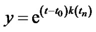
At  then
then  and the solution of Euler method (3.33) is
Then we can define the error
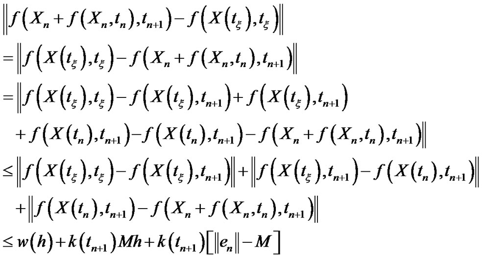
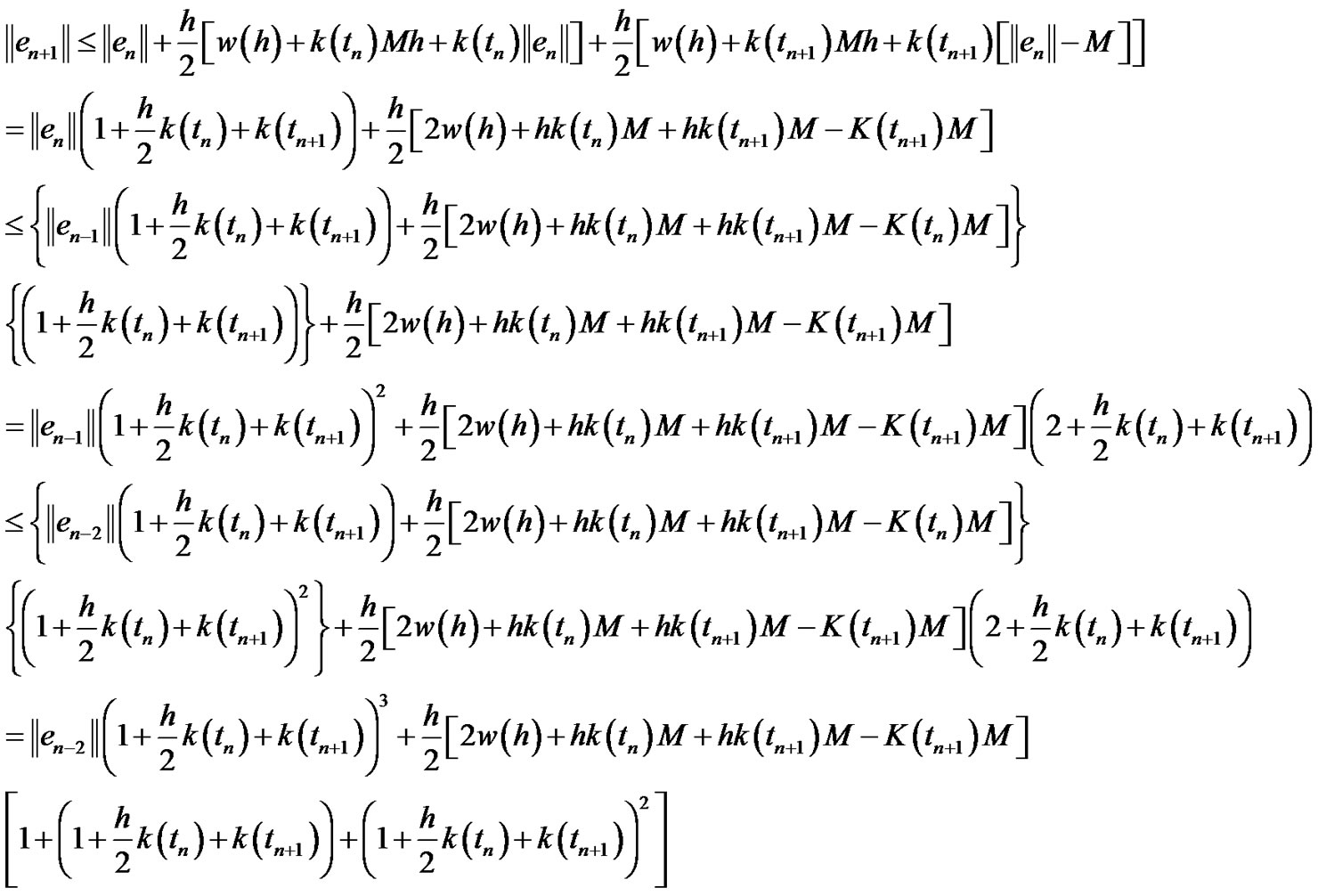
By (3.33) and (3.36) it follows that
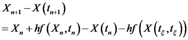
This implies

Hence
 (3.37)
Since:
 (3.38)
Since the theoretical solution  is m.s. bounded in
 ,
, 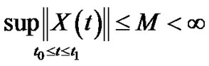 and Under hypothesis C1, C2 We obtain
• 
•  (*)
(*)
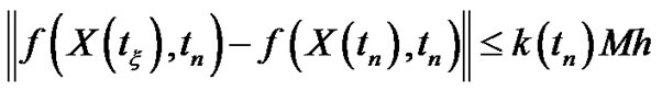
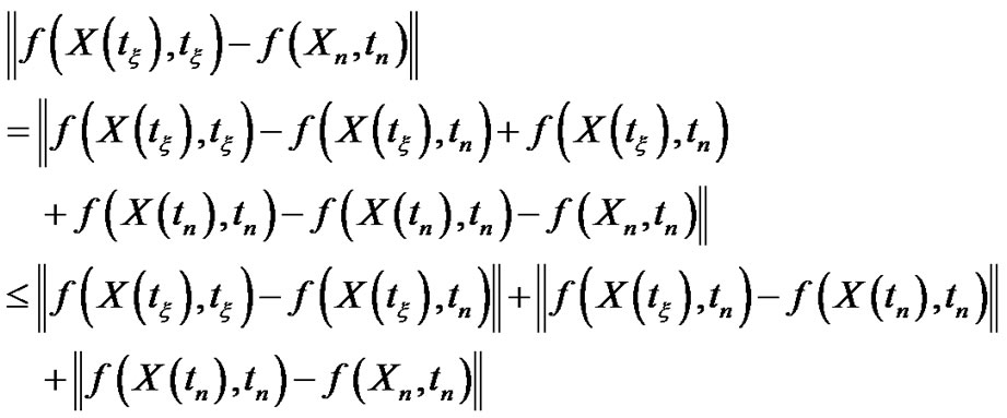
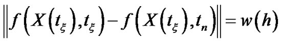
Since  is Lipschitz constant (from C2) and from Theorem (3.3.1) we have
 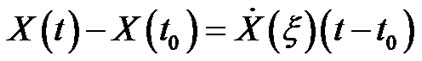 and note that the two points are
  and
and  in (*) then we have:
Since  and
and 
• 
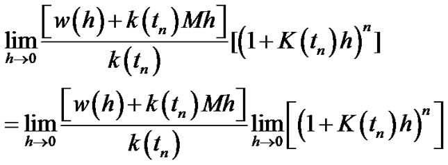
Then by substituting in (3.38) we have
 (3.39)
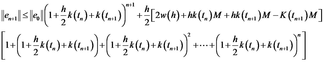
Then by substituting in (3.37) we have
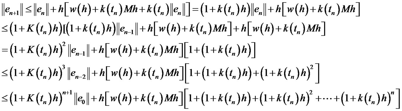
Since:
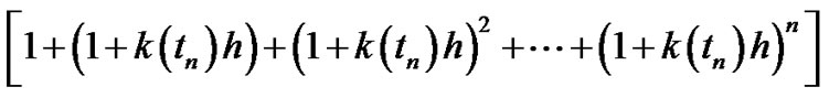
is geometrical sequence.
Then:
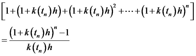
Then we get

Taking into account that  where
where
 .
.
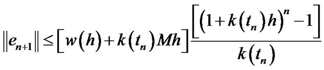
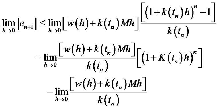 (3.40)
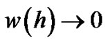
Note that:
The term: 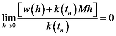 as
as
 (
(
 as
as )
)
(3.41)
And the second term:
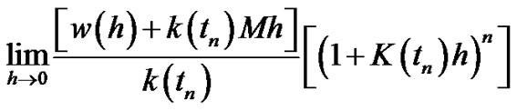
we have:
 (3.42)
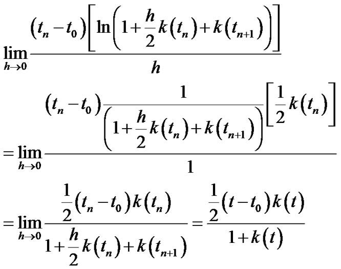
The first limit in (3.42) equal zero and:
The computation of 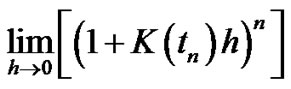 as follows:
Let  then by tacking the logarithm of the two sides we have:
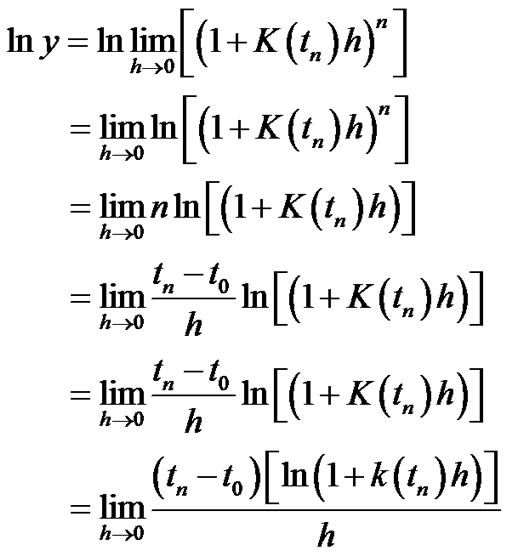
By using the (L’Hospital’s Rule):
 (3.43)
Then 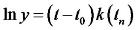 which implies that
 hence
hence
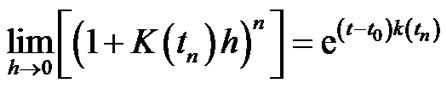
By substituting in (3.42):
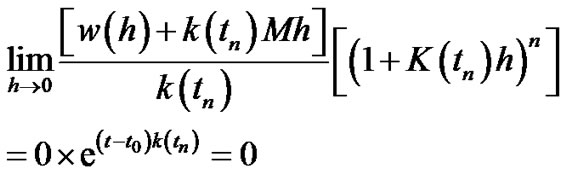 (3.44)
By substituting from (3.44) and (3.42) in (3.40) hence  i.e.,
i.e.,  converge in m.s to zero as
 hence
hence .
.
3.3. The Convergence of Runge-Kutta of Second Order Scheme for Random Differential Equations in Mean Square Sense
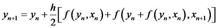
In this section we are interested in the mean square convergence, in the fixed station sense, of the random Runge-Kutta of second order method defined by
 (3.45)
where  and
and  are 2-r.v.’s,
  ,
,  and f:
 ,
,  satisfies the following conditions:
C1:  is randomly bounded uniformly continuousC2:
  satisfies the m.s. Lipschitz condition
where
 (3.46)
Note that under hypothesis C1 and C2, we are interested in the m.s. convergence to zero of the error
 (3.47)
where  is the theoretical solution 2-s.p. of the problem (3.22),
 .
.
Taking into account (3.22), and Theorem (3.3.1), one getsSince from (3.22) we have at  then
then

Note  and we can use
  instead of
And from Theorem (3.3.1) at  then we obtain
Note that we deal with the interval 
 and hence
  was the starting in the problem (3.22) and here
  is the starting and since Euler method deal with solution depend on previous solution and if we have
  instead of
 we can use
  instead of
  then the final form of the problem (3.22) is
 , for some
(3.48)
Now we have the solution of problem (3.22) is 
At  then
then  and the solution of Runge-Kutta of 2 order method (3.45) is
Then we can define the error

By (3.45) and (3.48) it follows that

Then we obtain:

By taking the norm for the two sides:
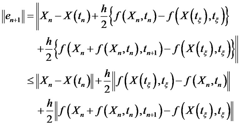 (3.49)
Since:
 (3.50)
Since the theoretical solution  is m.s. bounded in
 ,
,  and Under hypothesis C1, C2 We have
• 
•  (*)
(*)
where  Is Lipschitz constant (from C2) and:
From Theorem (3.3.1) we have
 and note that the two points Are
  and
and  in (*) then

where 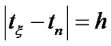 and
and 
• 
Then by substituting in (3.50) we have
 (3.51)
And another term:
Since:
• 
• 
where . Is Lipschitz constant (from C2) and:
From Theorem (3.3.1) we have
 and note that the two points are
 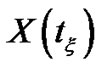 and
and  in (*) then we have:

where  and
and 
And the last term:

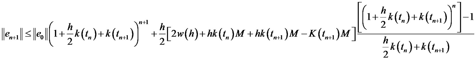
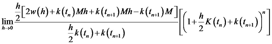
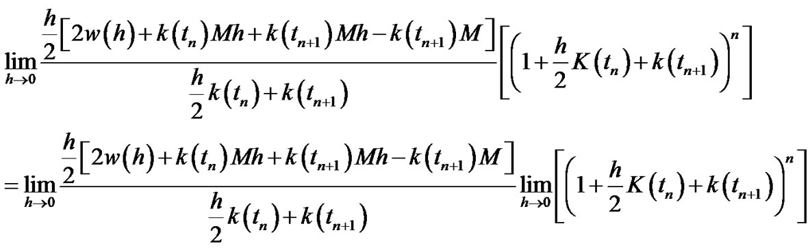
Then by substituting in (3.49) we have
Then we have:
Since:
is geometrical sequence then we have:
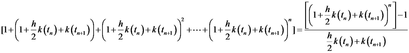
Then we get:
Taking into account that  where
where


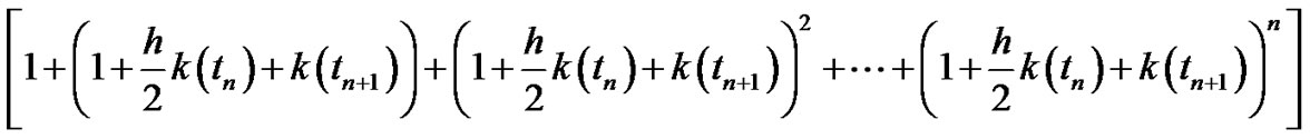
 (3.52)
Note that:
The term:
and the second term:
we have:
 (3.53)
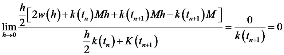
The first limit in (3.53) equals zero and:
The computation of
 is as follows:
Let  then by tacking the logarithm of the two sides we have:
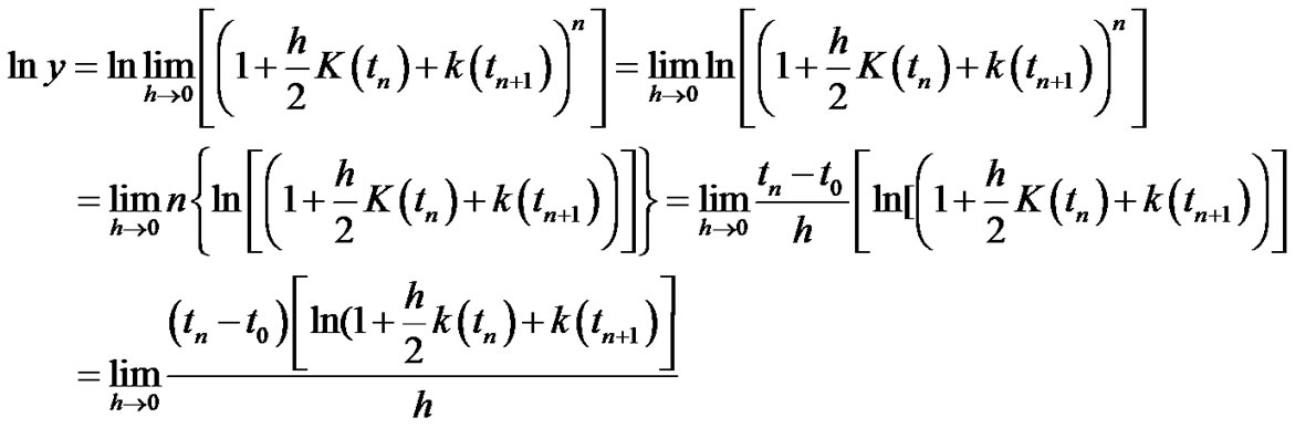
By using the (L’Hospital’s Rule):
 (3.54)
 Then
Then 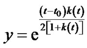 hence:

By substituting in (3.53):
 (3.55)
By substituting from (3.55) and (3.53) in (3.51) then we obtain 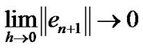 i.e.
i.e.  converges in m.s to zero as
  hence
hence 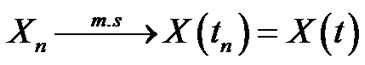
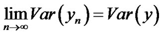
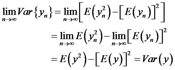
4. Some Results
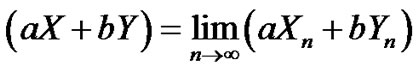
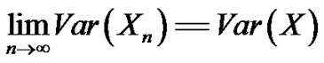
Theorem 4.1
Let {Xn, n = 0, 1, ···}, {Yn, n = 0, 1, ···} be sequences of 2-r.v’s over the same probability space and let a and b be deterministic real numbers.
Suppose:  and
and 
Then:
1) 
2) 
3) 
4) 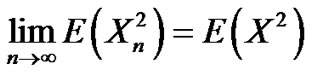
5) 
Definition 4.1 [13]. “The convergence in probability”
A sequence of r.v’s  converges in probability to a random variable
  as
as  if
if

Definition 4.2 [13]. “The convergence in distribution”
A sequence of r.v’s  converge in distribution to a random variable
  as
as  if
if

Lemma (4.1) [13]
The convergence in m.s implies convergence in probability
Lemma (4.2) [13]
The convergence in probability implies convergence in distribution
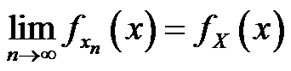
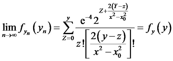
Theorem 4.2
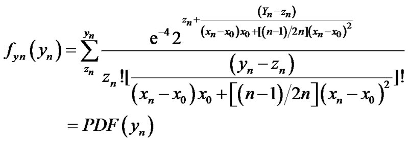
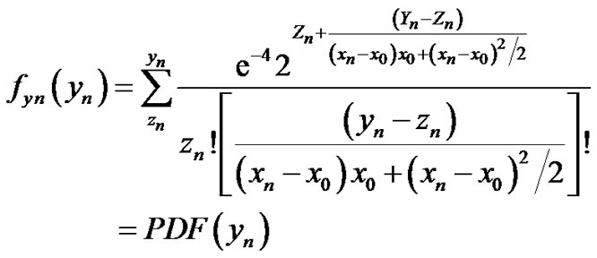
If 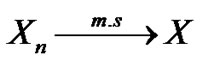 then PDF of
  PDF of
  i.e.;
i.e.; 
Proof Since we have shown that If  then
then

i.e., if  then
then 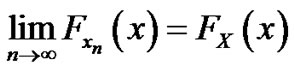
Then we have:  then
then
5. Numerical Examples
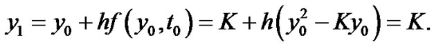
Example (5.1)
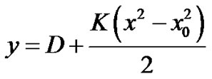
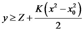
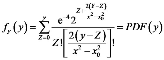
The differential equation with random term in it and random initial condition
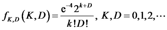
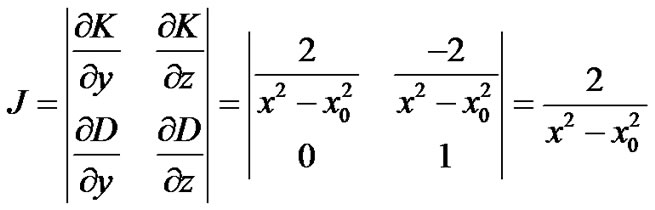
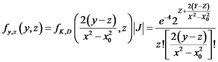
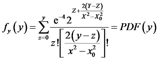
K, D are independent Poisson random variables with joint PDF
1) The exact solution,
2) The numerical solution
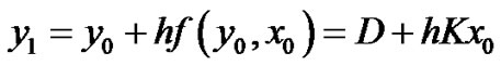
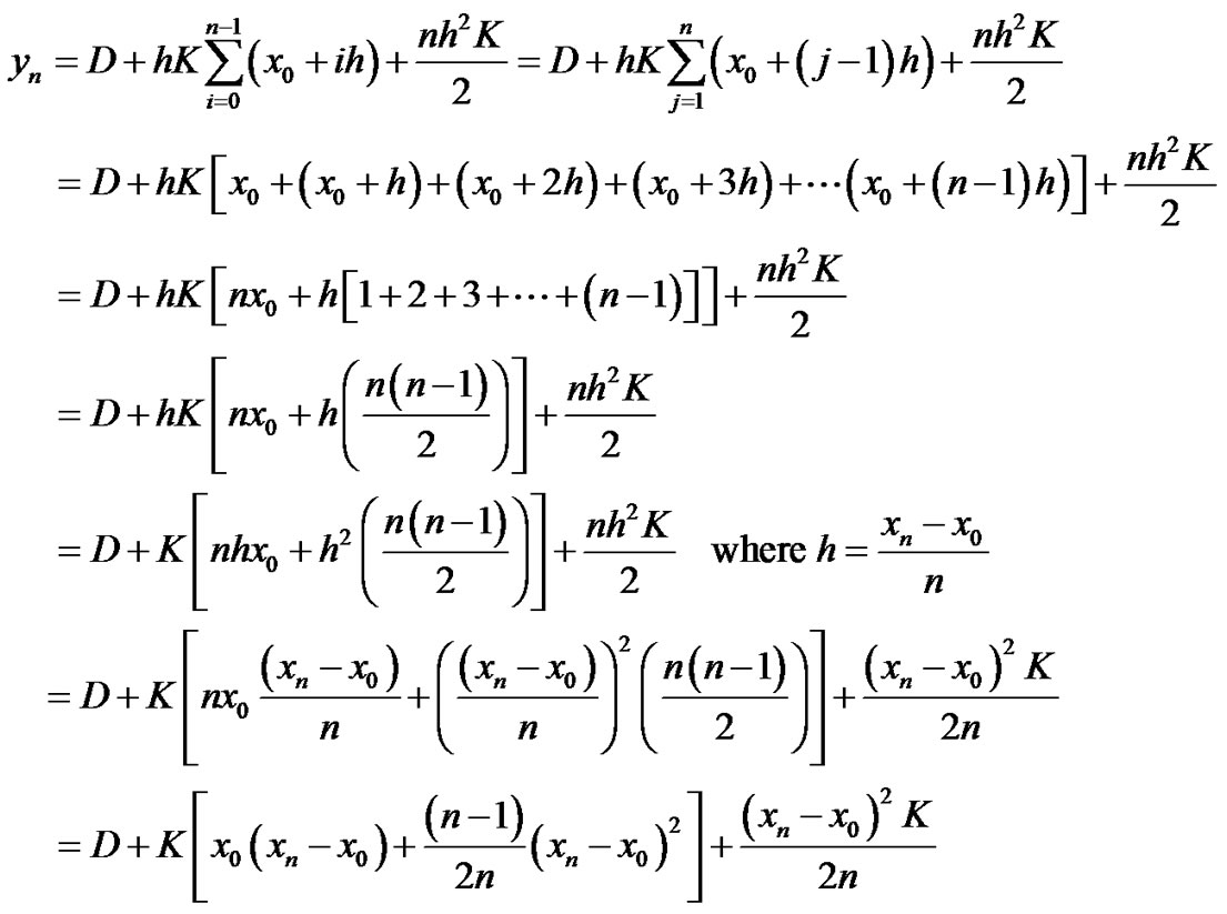
Using the Random Euler Method:
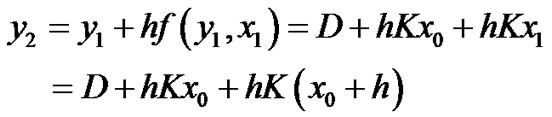
at n = 1
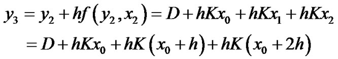
at n = 2
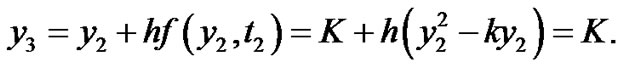
at n = 3
at n = 4

and so on…
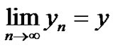
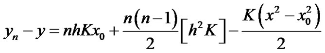
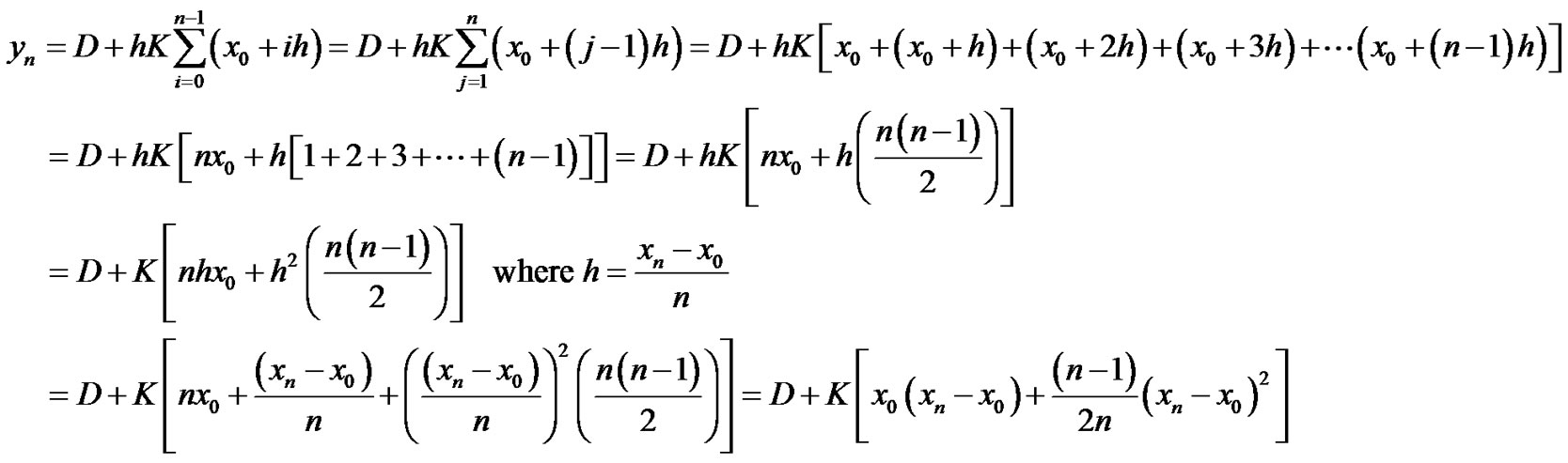
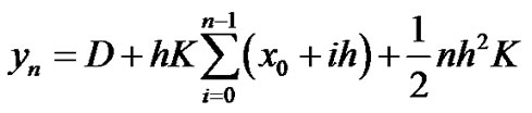
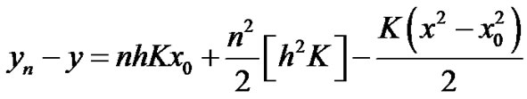
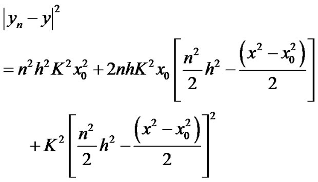
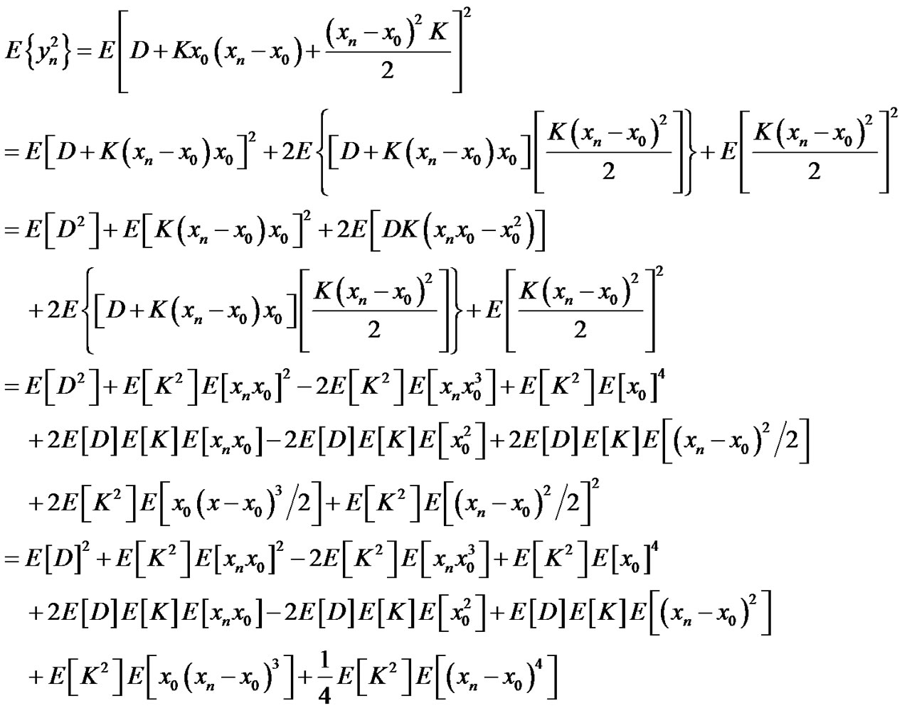
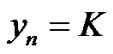
Then the general numerical solution is

i.e.,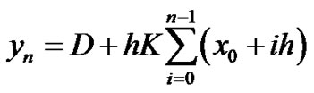 .
.
This can be written in another form:
 .
.
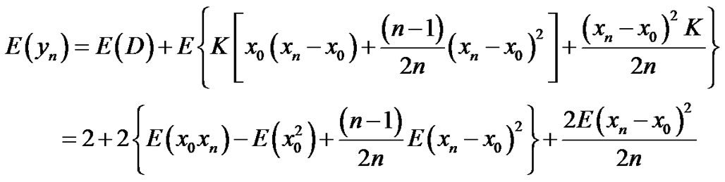
We can prove that:
1) 
Proof Since  (if and only if)
Then:
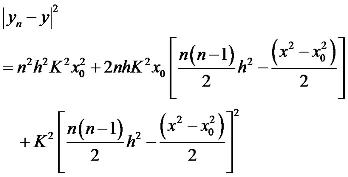
where 


i.e; 
We can verify theorem (4.1) as follows
2) 
Proof

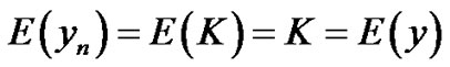
Then:
i.e.;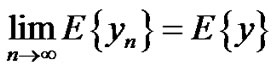 .
.
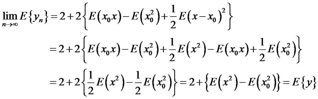
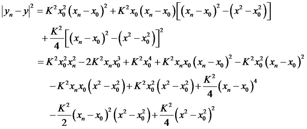
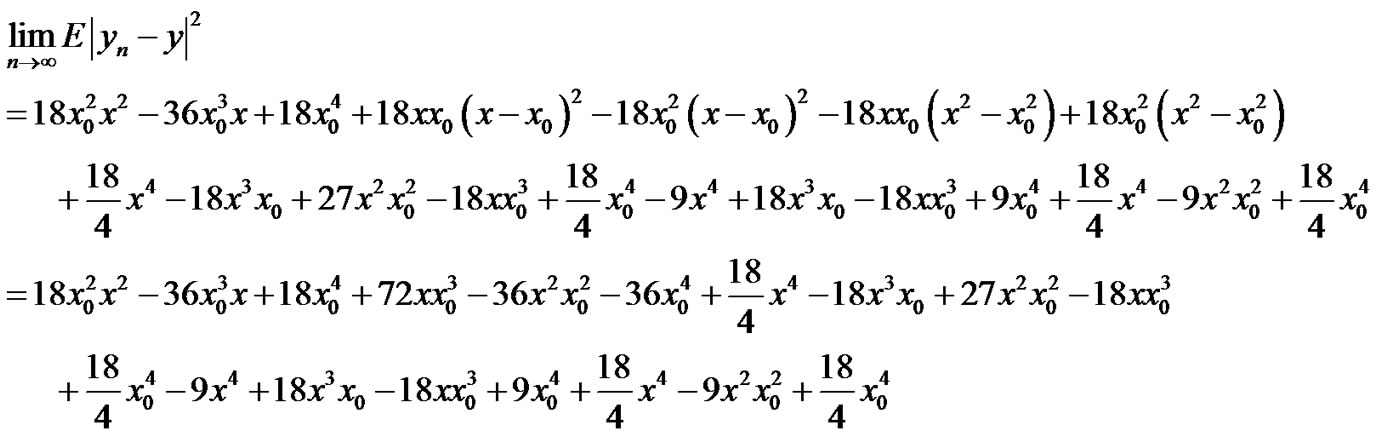
3) 
Proof Since 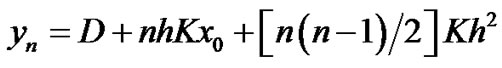
Then we have:
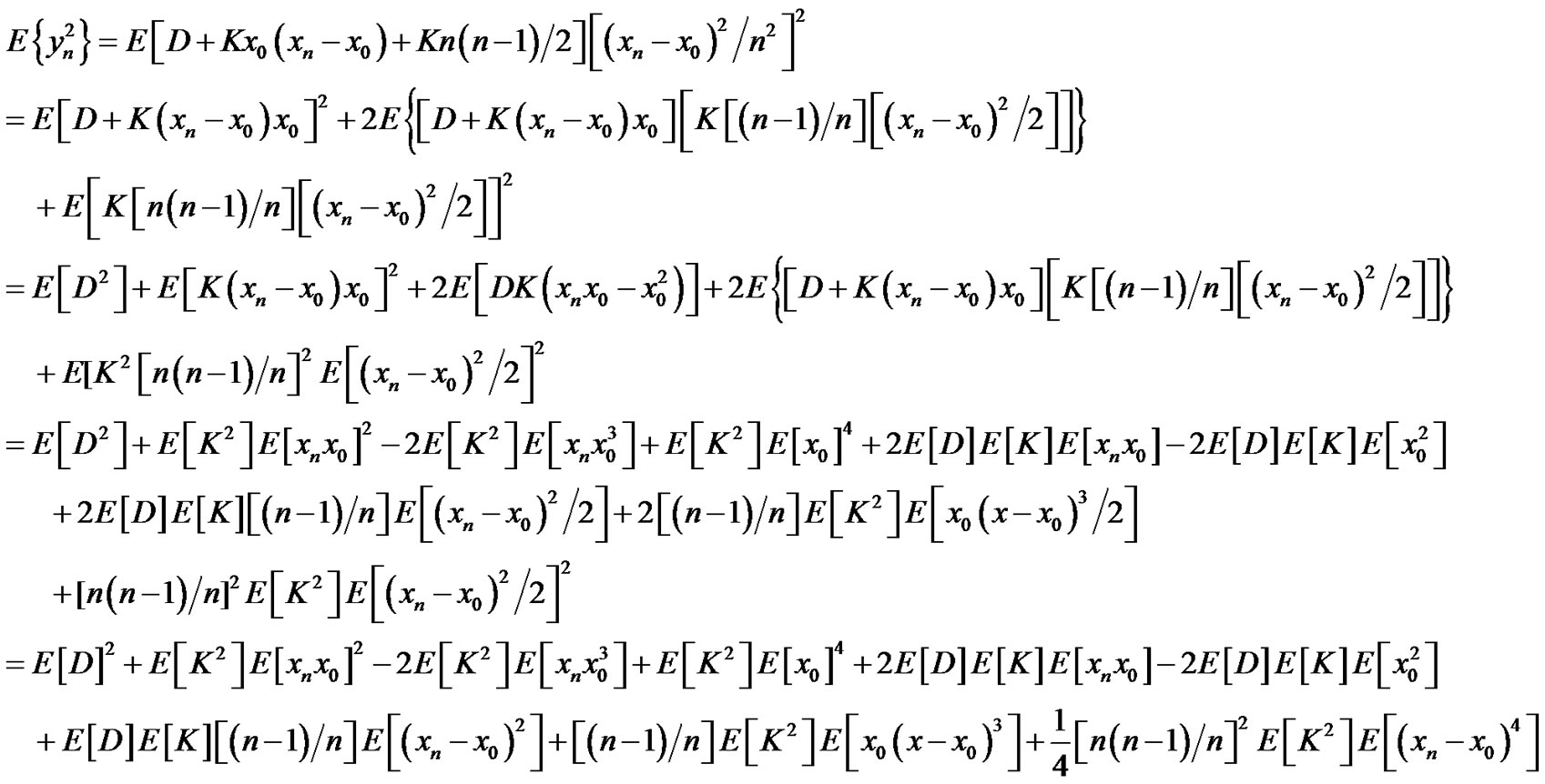
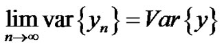
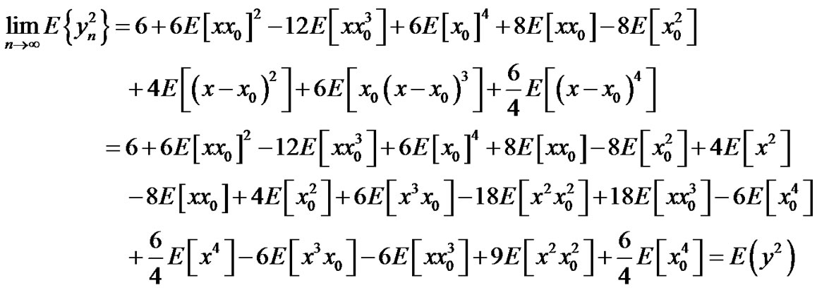
Then by taking the limit:
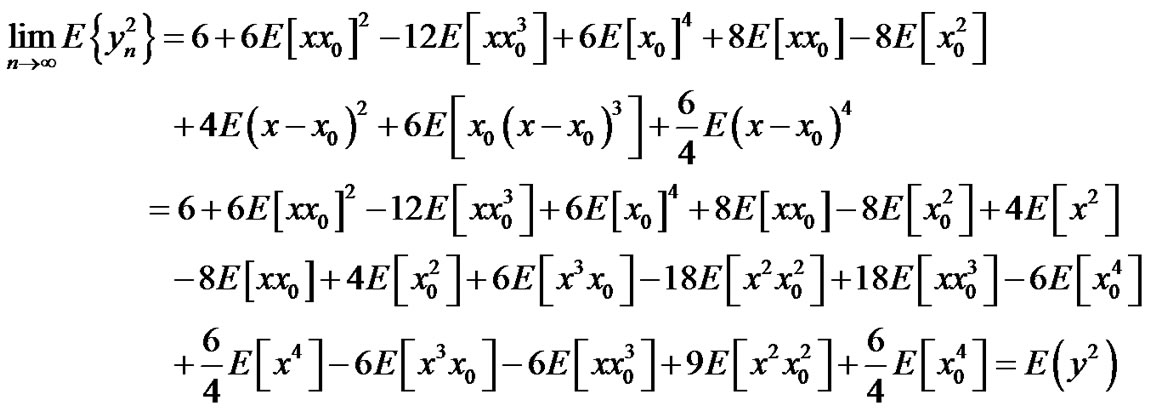
i.e. .
.
4) 
Proof

i.e., .
.
5) 
Proof Since 
Let us define Z = D. Then the inverse transformation is:
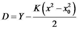 , D = Z then we have D = Z and
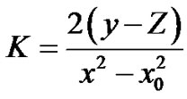
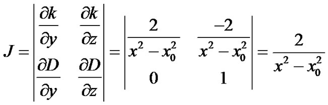
Then:

Since  then
then  hence
hence
 .
.
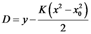
For a numerical solution:
since 
Let  then
then 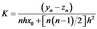
Then:


where 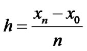
Then by taking the limit we have
i.e.; 
B. Using the Random Runge-Kutta method:
 at n = 0

At n = 1
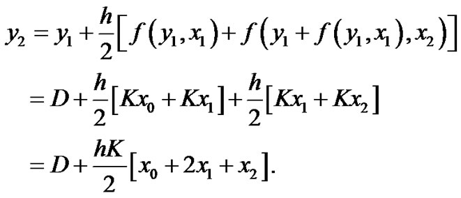
At n = 2
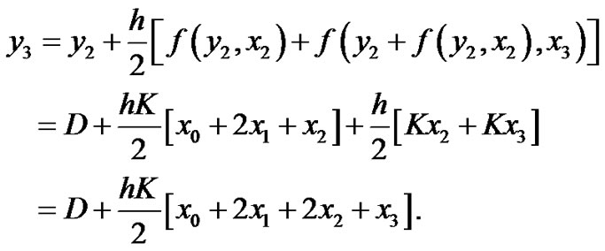
Then the general solution is:
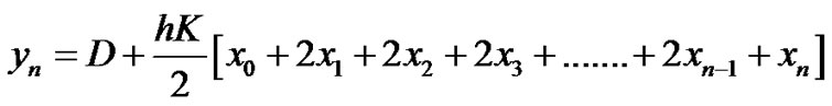 ,
,
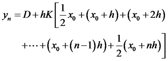 ,
,

 .
.
This can be written in another form:
 .
.
We can prove that:
1) 
Proof
Since  (if and only if)
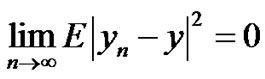
where 
i.e.; .
.
Verification of Theorem (4.1):
2) 
Proof

i.e.; .
.
3) 
Proof Since 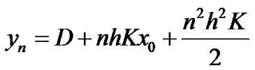 then:
then:
i.e.;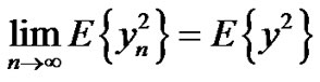 .
.
4) 
Proof
i.e. 
5) 
Since 
Let us define Z = D. Then the inverse transformation is:
 D = z then we have D = z and
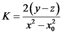
Since  then
then  this implies

 .
.
Numericallysince 
Let  then
then 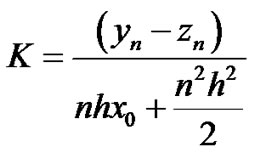


 where
where 

i.e.; .
.
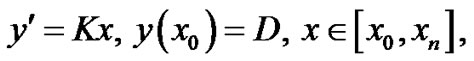
Example (5.2)
Solve the problem

The exact solution

The numerical solution by the Euler method:
AT n = 1
At n = 2

At n = 3
And so on….
Then the general numerical solution: .
.
It is clear that:
1) 
Since 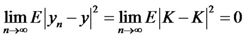
Verification of Theorem (4.1)
It is clear that:
2) 
3) 
Since 
4) 

5) 
 Then
Then  which implies

 Then
Then  which implies

Then: 
6. Conclusions
The initially valued first order random differential equations can be solved numerically using the random Euler and random Runge-Kutta methods in mean square sense. The existence and uniqueness of the solution have been proved. The convergence of the presented numerical techniques has been proven in mean square sense. The results of the paper have been illustrated through some examples.
7. References
[1] K. Burrage and P. M. Burrage, “High Strong Order Explicit Runge-Kutta Methods for Stochastic Ordinary Differential Equations,” Applied Numerical Mathematics, Vol. 22, No. 1-3, 1996, pp. 81-101. doi:10.1016/S0168-9274(96)00027-X
[2] K. Burrage and P. M. Burrage, “General Order Conditions for Stochastic Runge-Kutta Methods for Both Commuting and Non-commuting Stochastic Ordinary Equations,” Applied Numerical Mathematics, Vol. 28, No. 2-4, 1998, pp. 161-177. doi:10.1016/S0168-9274(98)00042-7
[3] J. C. Cortes, L. Jodar and L. Villafuerte, “Numerical Soluion of Random Differential Equations, a Mean Square Approach,” Mathematical and Computer Modelling, Vol. 45, No. 7, 2007, pp. 757-765. doi:10.1016/j.mcm.2006.07.017
[4] J. C. Cortes, L. Jodar and L.Villafuerte, “A Random Euler Method for Solving Differential Equations with Uncertainties,” Progress in Industrial Mathematics at ECMI, Madrid, 2006.
[5]H. Lamba, J. C. Mattingly and A. Stuart, “An adaptive Euler-Maruyama Scheme for SDEs, Convergence and Stability,” IMA Journal of Numerical Analysis, Vol. 27, No. 3, 2007, pp. 479-506. doi:10.1093/imanum/drl032
[6] E. Platen, “An Introduction to Numerical Methods for Stochastic Differential Equations,” Acta Numerica, Vol. 8, 1999, pp. 197-246. doi:10.1017/S0962492900002920
[7] D. J. Higham, “An Algorithmic Introduction to Numerical Simulation of SDE,” SIAM Review, Vol. 43, No. 3, 2001, pp. 525-546. doi:10.1137/S0036144500378302
[8] D. Talay and L. Tubaro, “Expansion of the Global Error for Numerical Schemes Solving Stochastic Differential Equation,” Stochastic Analysis and Applications, Vol. 38, No. 4, 1990, pp. 483-509. doi:10.1080/07362999008809220
[9] P. M. Burrage, “Numerical Methods for SDE,” Ph.D. Thesis, The University of Queensland, 1999.
[10] P. E. Kloeden, E. Platen and H. Schurz, “Numerical Solution of SDE Through Computer Experiments,” Second Edition, Springer, Berlin, 1997.
[11] M. A. El-Tawil, “The Approximate Solutions of Some Stochastic Differential Equations Using Transformation,” Journal of Applied Mathematics and Computing, Vol. 164, No. 1, 2005, pp. 167-178. doi:10.1016/j.amc.2004.04.062
[12] P. E. Kloeden and E. Platen, “Numeical Solution of Stochastic Differential Equations,” Springer, Berlin, 1999.
[13] T. T. Soong, “Random Differential Equations in Science and Engineering,” Academic Press, New York, 1973.