American Journal of Computational Mathematics
Vol. 3 No. 2 (2013) , Article ID: 33541 , 7 pages DOI:10.4236/ajcm.2013.32019
Error Estimation and Assessment of an Approximation in a Wavelet Collocation Method
University of Applied Science, Darmstadt, Germany
Email: michael_050485@yahoo.com
Copyright © 2013 Marco Schuchmann, Michael Rasguljajew. This is an open access article distributed under the Creative Commons Attribution License, which permits unrestricted use, distribution, and reproduction in any medium, provided the original work is properly cited.
Received January 17, 2013; revised February 25, 2013; accepted March 23, 2013
Keywords: ODE; Sinc Collocation; Shannon Wavelet; Wavelet Collocation; Error Estimation
ABSTRACT
This article describes how to assess an approximation in a wavelet collocation method which minimizes the sum of squares of residuals. In a research project several different types of differential equations were approximated with this method. A lot of parameters must be adjusted in the discussed method here. For example one parameter is the number of collocation points. In this article we show how we can detect whether this parameter is too small and how we can assess the error sum of squares of an approximation. In an example we see a correlation between the error sum of squares and a criterion to assess the approximation.
1. Introduction
In the wavelet theory a scaling function  is used, which has properties that are defined in the MSA (multi scale analysis). Through the MSA we know, we can construct an orthonormal basis of a closed subspace
 , where
  belongs to a sequence of subspaces with the following property:
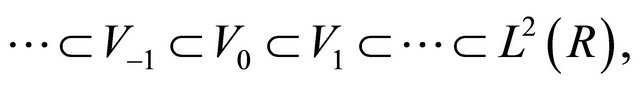
 is an orthonormal basis of
  with
with
 .
.
We use the following approximation function:
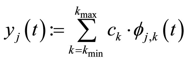 , with
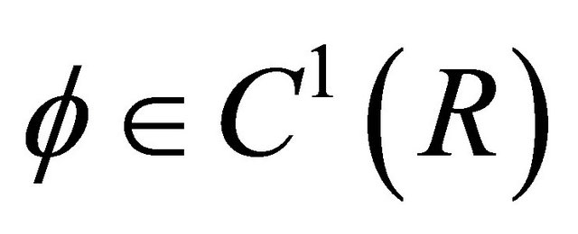 .
.
 and
and  depend on the approximation interval
 .
.
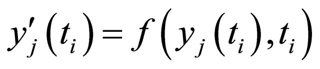
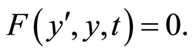
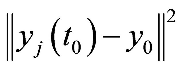
Now we can approximate the solution of an initial value problem 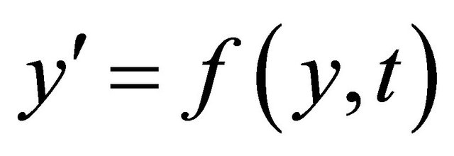 and
and  by minimizing the following function (
 is the Euklid norm)
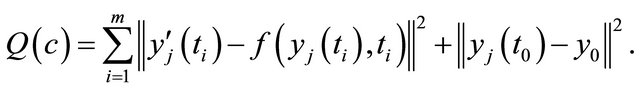 (1)
(1)
For 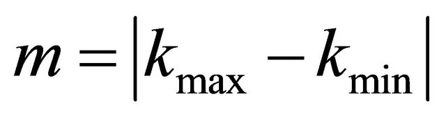 we get an equivalent problem:
 , with
  and
and .
.
The advantage of calculating  by minimizing
  is that we can choose more collocation points
  as shown in the following example. In that case we apply the least squares method to calculate
 . Many simulations had shown that if
  was very small then the approximation yj would be good. An even better criterion for a good approximation
  is
is  (see (3)). Moreover, the equations have been ill-conditioned in several examples.
Analogously we could use boundary conditions instead of the initial conditions. This method can be even used analogously for PDEs, ODEs of higher order or DAEs, which have the form
If  is an ODE system, then we use the approximation function:
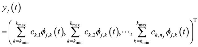
For the i-th component of the solution y, we use the notation  as usual. We use for the i-th component of
  the notation
 , in order not to lead to a confusion with the approximation
  out of
 , so it will be always distinguished whether the approximation
  or the i-th component of
  is used.
We use the collocation points , with
  and
and
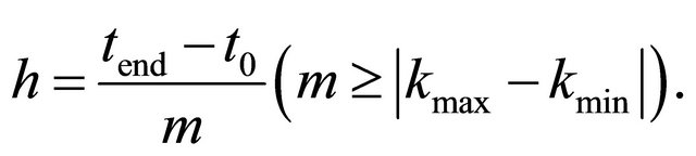 (2)
(2)
Simulations have shown that even with  we get good approximations.
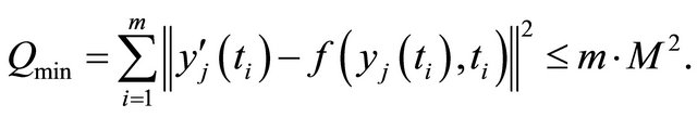
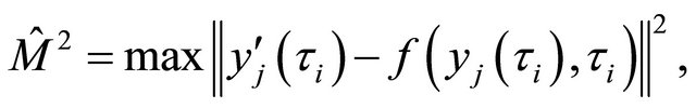
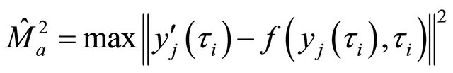
For the assessment of the approximation we use the value , with
 (3)
(3)
 ,
,  and
and  is an integer. For big
  we should weight
  with
with .
.
Remarks 1:
1) We get

for , because of:
Analogously for smaller .
.
2) The sums in (1) and (3) could start with , too.
3)  in (1) could also be used as a constraint if the initial value should be fulfilled. But in all good approximations,
  was very small.
In the examples we use the Shannon wavelet. Although it has no compact support and no high order, in many examples and simulations we got a much better approximation than using other wavelets (f.e. Daubechies wavelets of order 5 to 8), even with a small n. The Meyer wavelet yields good results, too.
We even get a good extrapolation outside the interval .
.
Example 1:
1) We use the following ODE

The exact solution is .
.
We approximated the solution on the interval  and chose
 , like in all examples.
With  we could see in all our simulations, if the approximation was good. We got a linear relationship between
  and
and . In Figure 1 we see the graph of a linear regression (with an R squared of 0.991196) of
  against
  with the points
 , which have been calculated with different
 and
and 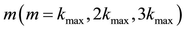 with the ODE and I of the example 1.
 is the mean squared error
 with
with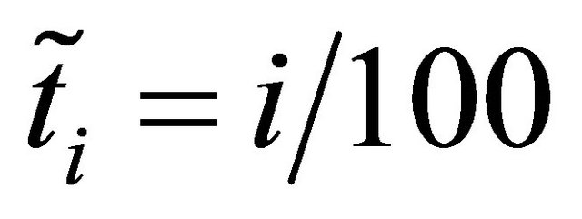 .
.
Now we see a regression table (Table 1) of  on
on , which shows a linear dependency in our example and the graph of the linear regression function.
Here is a graph of the regression function and the graphs of the functions yi and  for j = 0, kmax = 15 and
  on the approximation interval
  (see Figures 2 and 3) and on the interval
  (see Figures 4 and 5). In Figures 4 and 5 we see that we get even a good extrapolation.

Figure 1. Linear regression plot of  against
 .
.
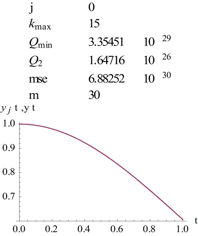
Figure 2. Graph of , kmax = 15, m = 30.
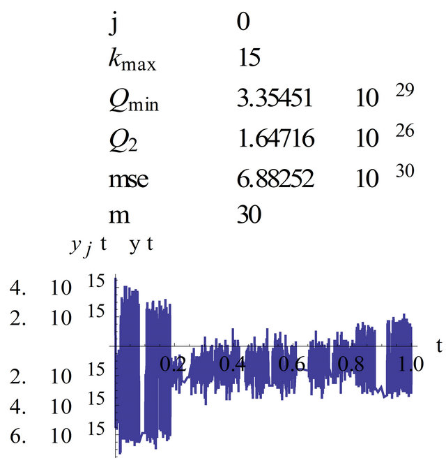
Figure 3. Graph of , kmax = 15, m = 30.

Figure 4. Graph of , kmax = 15, m = 30.
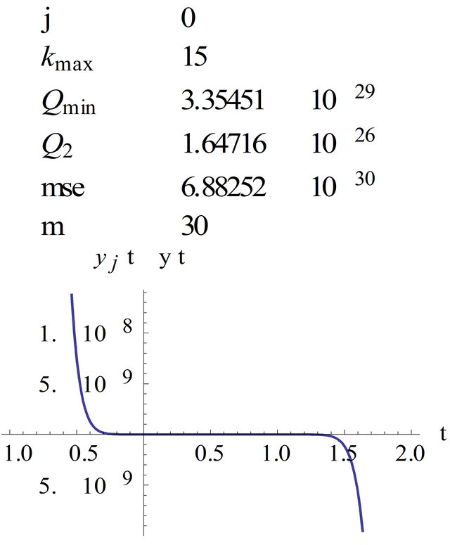
Figure 5. Graph of , kmax = 15, m = 30.

Table 1. Linear regression table of  on
on .
.
2. Error Estimation and Assessment of the Approximation
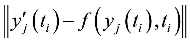
In the example we used the Shannon wavelet. For this wavelet we have additional information about the error in the Fourier space from the Shannon theorem. For a good approximation with a small j the behavior of  with growing
  is important, because (if yi is an orthogonal projection from y on Vj and
 )
)
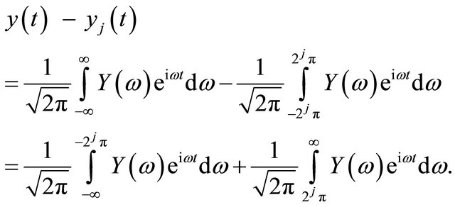
With the Parseval theorem we get

so
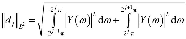
With the Riemann-Lebesgue theorem we get:

For the approximation error the decay behaviour of the detail coefficients  is important:

On the other side: we have got in many simulations with the Shannon wavelet better approximations (with the described collocation method) than with higher order wavelets.
Remarks 2:
1) For a theoretical multi resolution analysis we could consider  instead of
 , because when
  is in
is in  then
then  is in
is in , if we need an approximation on
 . Here
  is the indicator function of the interval
 .
.
2) For interpolating wavelets there are a number of publications with error estimates and also for the approximation of the solutions of initial value problems and boundary value problems (for ordinary and partial differential equations) see [1,2], as well as to the sinc collocation method (see [3-5]) with special collocation points (“sinc grid points”, see [5]).
Theorem 1 (for the decay behaviour):
The wavelet  has the order
 ,
,  with
with  and
and  is Lipschitz continuous. Then exists a
  independent from
  with
with
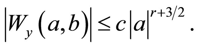
 is the wavelet transform of
  with
with

A proof is in [6]. So we get for the detail coefficients an appraisal because

and so

Now we saw that the decay of the detail coefficients depends on the order of a wavelet.
From the Gilbert-Strang Theory (see [7]) we know additionally an upper bound of the approximation error in dependency of the order : if the wavelet is of order
  then the approximation error has the order
 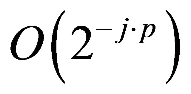 if
if  and (if
  is an orthogonal projection from
  on
on  and
and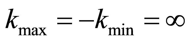 )
)
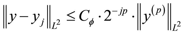 .
.
If a wavelet is of order  the scaling function
  even has an interpolation property, because then we can construct the functions
  with
with 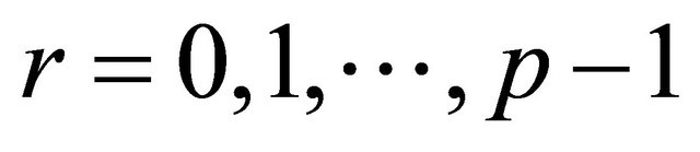 over a linear combination of
  (see [7]). That’s also a property of the so called interpolating wavelets. For interpolating wavelets we find error estimations in [8] and [9].
Remarks 3:
1) Error estimations for the sinc collocation with a transformation can be found in [4] and [5].
2) Although the approximation error is depended on the order of a wavelet in many simulations the Shannon wavelet led to much better approximations than Daubechies wavelets of higher order, if the approximation function  was calculated by minimizing the sum of squares of residuals Q. Even when comparing the extrapolations the Shannon wavelet was significantly better.
The reason is, that we do not calculate an orthogonal projection on  like in the appraisal above and the function y is in general case not quadratic integrabel on R (we consider only a compact interval I).
The following appraisal takes account of the fact that we calculate the approximation function by the minimization of Q. We first need a theorem, which follows from the Gronwall-Lemma.
Theorem 2:
Assumptions: we have a initial value problem  with
with  and
and
 (4)
(4)
and
 (5)
(5)
Then we get for :
:

For a proof see [10].
Theorem 3:
With the assumptions from Theorem 2 we get (if 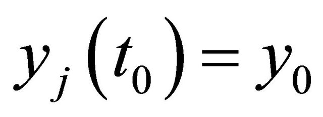 ):
):
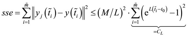
So we get the follow inequality for , which is used in the example 2:
 (6)
(6)
 depends on
  and
and 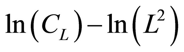 only on the initial value problem and the collocation points. We write
  instead of
 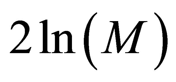 because in example 2 we set
  on the x-axes so we have a comparison with example 1 where we set
  on the x-axes.
Remark 4:
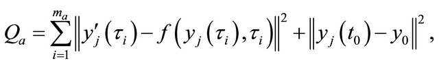
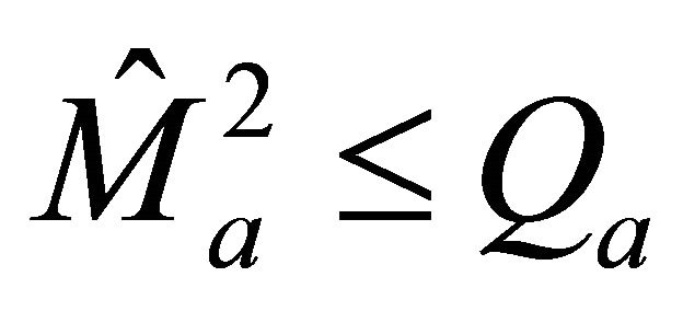
We get with 
If additionally 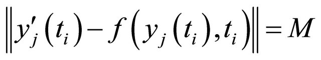 for one (or more)
 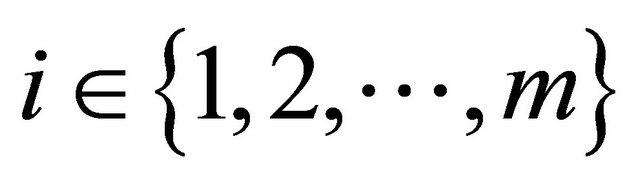 we get:

This is analogously right for  instead if
  with
with

and 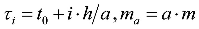 and an integer
 . Qa is an upper bound for
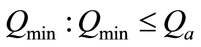 . With
  we could assess in all simulations the quality of an approximation and in linear regressions from
  on
on  we got in almost all simulations a
  (R squared) greater than 0.99 (see next example). Only if all approximations have been bad, then
  was less than 0.99 (but we still have a dependency). If
  is the exact solution, then
 . Because we get not only a approximation with points (we get a approximation function
 ) we must not calculate a second minimization for the calculation of
 .
.
 will be in general (for
 ) less than M, because we use the collocations points ti and so
  is very small at these points (see the next graphic).
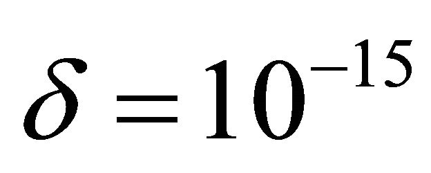
  was in many good simulations less than 10−16.
In many simulation  is relative big between to collocation points (or at the edge of I if we start with i = 1 in the sum (1)).
In Figure 6 we see the graph of
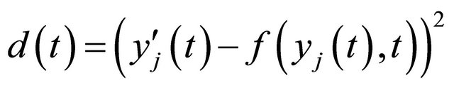
in example 1 for 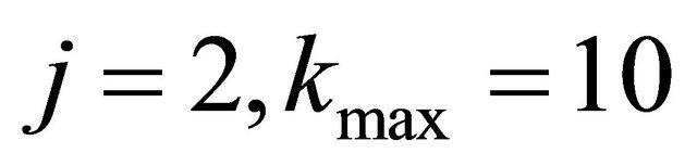 and
and . Here a too small
  results in a very bad approximation.
We see that  could be very small with a too small m, but
  is very big here. In the graph we see that d is very small at the collocation points
  but between them d is very big. That’s the reason because we could identify with
  a worse approximation in any our simulations. On the other hand a big
  is an indicative of a too small j.
So we can approximate M here with the maximum of  at the points
  with
with  like we do it in the next example.
Now we want to apply the result from theorem 2. Furthermore we will see a correlation between an approximation of  and
and  in this example like we saw it before between
  and
and .
.

Figure 6. Graph of d.
Example 2:
We use the initial value problem and the approximations with the different parameters ,
,  and m of example 1. If
  than follows from theorem 2 (under the assumptions from this theorem):

Here we get (see (6)):

We now apply a linear regression of  on
on  with the approximation
from M2 with  (the points from
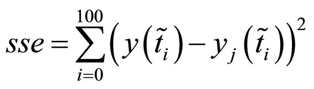
  beginning with
 ). sse and
  have been calculated with the points
  (and the summation indices
 ).
).
Here is the regression table (Table 2) (with a R squared of 0.986877).
In Figure 7 we see a graph from  (in red), the graph of the regression function (in blue) and the regression points
 .
.  was not considered (this means we set
 ) because it was very small.
Here are the graphs of  with
with ,
, 
and  in Figure 8. In most simulations
  was less than 10−16.
Generally we can use
 ,
,
 and
and  (with an integer
 ) for an approximation of
 . Here we know the following relation:
3. Conclusions
We defined a variable  with which you can evaluate an approximation. In many simulations and in the examples of this article we saw that we get good results with
 . A linear relationship between
  and
and  was shown in example 1. It is also shown that the approximation can be used to extrapolate outside the approximation interval.
Using Theorem 2 we derive an estimate (see theorem 3). Then it is shown how to detect a too great step size using . In example 2 we show that the deduced estimate represents a straight line (in the coordinate system with
  on the x-axes and
  on the yaxes), which runs approximately parallel to the regression line (it is approximately parallel because the regression function is an estimation, theoretically it must be parallel because it cannot cross the upper bound line). In a research project we got analogous results in many
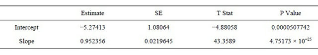
Table 2. Regression table of  on
on .
.
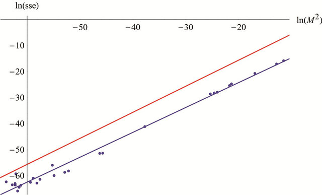
Figure 7. Linear regression plot of  against
 .
.
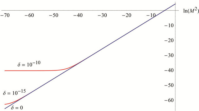
Figure 8. Graphs of  with
with ,
,  and
and .
.
simulations, even with systems and higher order odes.
It is shown that  (the size of the estimate) can be approximated via
 , and this approximation has
  as upper bound. The regression of the points
 returns a slightly larger
  than the regression with the points
 . As a consequence, Q2 is well suited to assess, especially as you can estimate the approximation of
  with Q2 and in Q2 more information is included. Moreover we can compare Q2 with
  to assess the approximation (see Figure 6).
REFERENCES
- O. V. Vasilyev and C. Bowman, “Second-Generation Wavelet Collocation Method for the Solution of Partial Differential Equations,” Journal of Computational Physics, Vol. 165, No. 2, 2000, pp. 660-693. https://wiki.ucar.edu/download/attachments/41484400/vasilyev1.pdf doi:10.1006/jcph.2000.6638
- S. Bertoluzza, “Adaptive Wavelet Collocation Method for the Solution of Burgers Equation,” Transport Theory and Statistical Physics, Vol. 25, No. 3-5, 2006, pp. 339-352. doi:10.1080/00411459608220705
- T. S. Carlson, J. Dockery and J. Lund, “A Sinc-Collocation Method for Initial Value Problems,” Mathematics of Computation, Vol. 66, No. 217, 1997, pp. 215-235. doi:10.1090/S0025-5718-97-00789-8
- K. Abdella, “Numerical Solution of Two-Point Boundary Value Problems Using Sinc Interpolation,” Proceedings of the American Conference on Applied Mathematics, Applied Mathematics in Electrical and Computer Engineering, 2012, pp. 157-162.
- A. Nurmuhammada, M. Muhammada, M. Moria and M. Sugiharab, “Double Exponential Transformation in the Sinc-Collocation Method for a Boundary Value Problem with Fourth-Order Ordinary Differential Equation,” Journal of Computational and Applied Mathematics, Vol. 162, No. 2, 2005, pp. 32-50. doi:10.1016/j.cam.2004.09.061
- C. Blatter, “Wavelets—Eine Einführung,” 2nd Edition, Vieweg, Wiesbaden, 2003.
- G. Strang, “Wavelets and Dilation Equations: A Brief Introduction,” SIAM Review, Vol. 31, No. 4, 1989, pp. 614- 627. doi:10.1137/1031128
- Z. Shi, D. J. Kouri, G. W. Wie and D. K. Hoffman, “Generalized Symmetric Interpolating Wavelets,” Computer Physics Communications, Vol. 119, No. 2-3, 1999, pp. 194-218. doi:10.1016/S0010-4655(99)00185-X
- D. L. Donoho, “Interpolating Wavelet Transforms,” Technical Report 408, Department of Statistics, Stanford University, Stanford, 1992.
- E. Hairer and G. Wanner, “Solving Ordinary Differential Equations I: Nonstiff Problems,” 2nd Edition, Springer, Berlin, 1993.