American Journal of Computational Mathematics
Vol.2 No.3(2012), Article ID:23183,6 pages DOI:10.4236/ajcm.2012.23026
The Best Finite-Difference Scheme for the Helmholtz Equation
1School of Mathematics and Computer Science, National University of Mongolia, Ulaanbaatar, Mongolia
2School of Mathematics, Mongolian University of Science and Technology, Ulaanbaatar, Mongolia
Email: v_ulzii@yahoo.com
Received June 6, 2012; revised August 8, 2012; accepted August 12, 2012
Keywords: The Best Finite-Difference Scheme for the Helmholtz and Laplace’s Equations
ABSTRACT
The best finite-difference scheme for the Helmholtz equation is suggested. A method of solving obtained finite-difference scheme is developed. The efficiency and accuracy of method were tested on several examples.
1. Introduction
The finite-difference method is a standard numerical method for solving boundary value problems. Recently, considerable attention has been attracted to construct a best (or exact) difference approximation for some ordinary and partial differential equations [1-3]. In this paper a best finite-difference method is developed for Helmholtz equation with general boundary conditions on the rectangular domain in R2. The method proposed here comes out from [4] and is based on separation of variables method and expansion of one-dimensional threepoint difference operators for sufficiently smooth solution. The paper is organized as follows. The statement of problem and the separation of variables method are considered in section 2. A detailed description of the best difference approximation to the Helmholtz equation in rectangular domain is given in section 3.
Section 4 is devoted to derive the best approximation for the given third kind boundary conditions. The method of solution for the obtained difference equations is considered in section 5 and numerical examples are given last section 6.
2. Statement of Problem
Let  be an open rectangular domain in Euclidean R2 space with boundary given by
 . The aim is to determine a function
 , satisfying equation
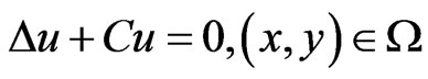 (2.1)
(2.1)
with boundary condition
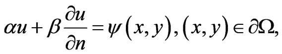 (2.2)
(2.2)
where C in (2.1) is a given number and  is the outward normal on
 .
.
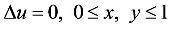
It is well known that the stabilized oscillation problems and diffusing processes in gas lead to the so called Helmholtz Equation (2.1) with a positive coefficient  The diffusing process in the moving field leads to the Equation (2.1) with negative coefficient
 . If C = 0 the Equation (2.1) leads to Laplace’s ones. Obviously, the properties of the solution of Equation (2.1) depend essentially upon the sign of the coefficient C in (2.1). We will assume that the problem (2.1), (2.2) has an unique and sufficiently smooth solution.
By virtue of variables method looking for the solution  of Equation (2.1), (2.2) in the form
 (2.3)
(2.3)
we arrive at equation
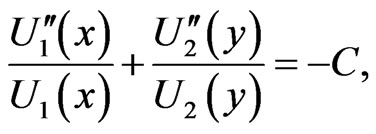
which is splitted into two independing equations
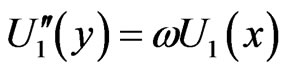 (2.4a)
and
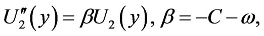 (2.4b)
where the unknown separation constant ω is to be found.
By virtue of (2.3) the boundary condition (2.2) is splitted info ones for  and
and 
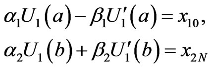 (2.5)
(2.5)
and
 (2.6)
(2.6)
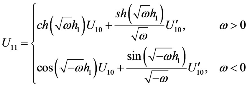
The solution of boundary value problem (2.4a), (2.5) is founded in a closed from
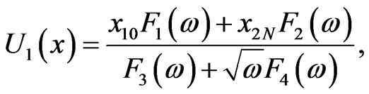 (2.7)
(2.7)
where
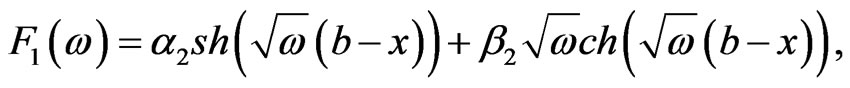
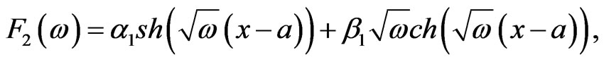

and
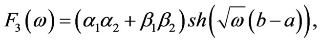
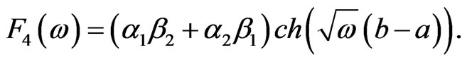
When ω < 0 the functions sh and ch in (2.7) are to be replaced by sin and cos respectively and ω replaced by –ω. Analogously, we can find the solutions of boundary value problem (2.4b) and (2.6) in closed form. Then from (2.3) and (2.7) clear, that the problem consists in determining the separation constant ω.
3. Construction of the Best Finite-Difference Equations
For the numerical solution of problem (2.1), (2.2) is introduced the uniform rectangular grid 
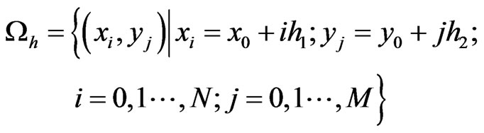
where  and
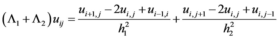
and  are the mesh sizes in the x and y directions respectively. Usually, the Equation (2.1) is approximated by the five-point difference equation
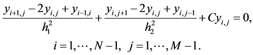 (3.1)
(3.1)
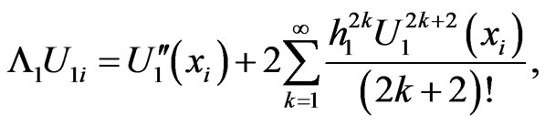
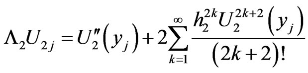
The local discretization error of the Equation (3.1) is of  order. Now we describe how to derive the best difference scheme for Equation (2.1). To this end, we consider expression
 (3.2)
(3.2)
where . If we denote by
  the values of
  the values of
  and
and  respectively, the using (2.3) the Equation (3.2) may be written as
 (3.3)
(3.3)
Due to smoothness assumption of solution  as well as, functions
  and
and  the Taylor series expansion yields
 (3.4a)
 (3.4b)
Because of (2.4) we have
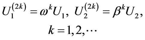 (3.5)
(3.5)
Taking into account (3.4), (3.5) in (3.3) it follows that
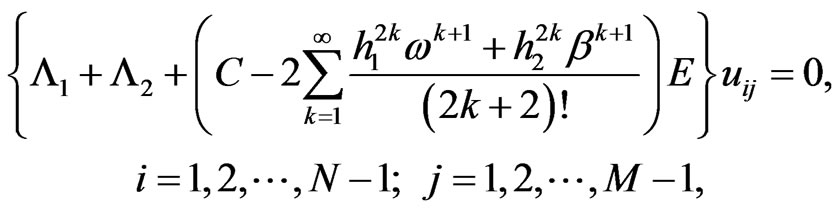 (3.6)
(3.6)
where E is unit operator. The difference Equation (3.6) contains unknown nonzero parameter ω and therefore it may be considered as a nonlinear equation with respect to the parameter ω and  The series in (3.6) may be expressed through analytical functions depending on the sign of quantities ω and β and thereby the Equation (3.6) can be rewritten as
 (3.7)
(3.7)
There are three cases:
1) Let  Then it is easy to show that
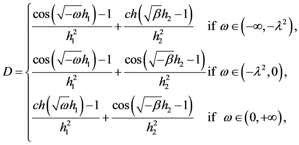 (3.8)
(3.8)
2) Let  In this case D is given by
 (3.9)
(3.9)
3) Let  In this case D is given by
 (3.10)
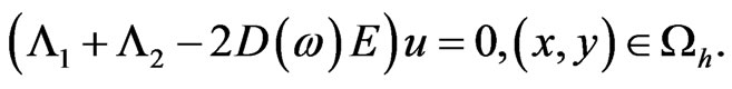
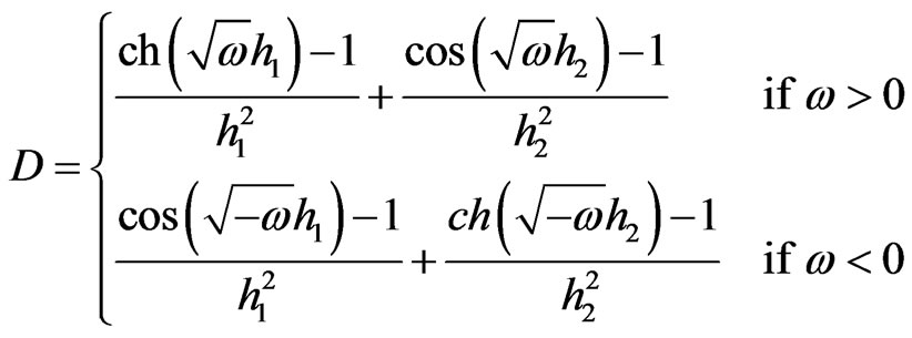
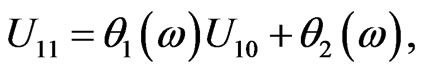
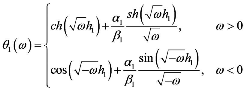
Thus we obtain the best (or exact) five-point difference Equation (3.7) for the Equation (2.1) (see, for example, Mickens [2] and Agarwal [1]). The function  in (3.7) can be presented as a sum of two ones, i.e.,
 (3.11)
where  and
and  correspond to the first and second terms in (3.8), (3.9) and (3.10) respectively.
4. The Best Finite-Difference Boundary Condition
Now we will derive a best difference boundary condition for (2.5), (2.6). Using (2.4) in the Taylor series expansion
we obtain
 (4.1)
(4.1)
If  in (2.5), then we have
 (4.2a)
If  then finding
  from (2.5) and substituting it in (4.1) we get
 (4.2b)
where  and
and  are given by
 (4.3a)
and
 (4.3b)
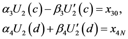
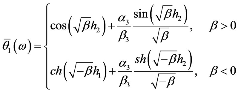
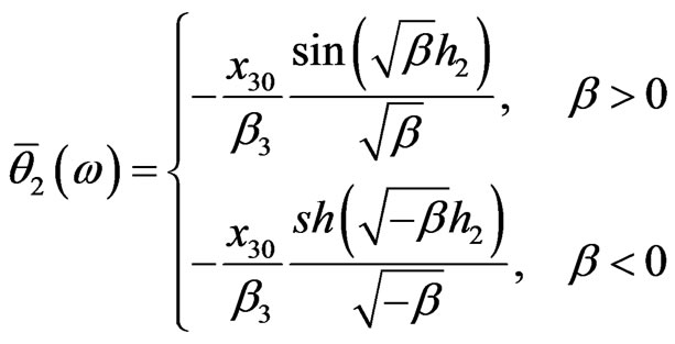
Analogously, it is easy to verify that the exact difference boundary condition for  at point
  is given by
 when
when  (4.4a)
 when
when  (4.4b)
where  and
and  are given by
 (4.5a)
and
 (4.5b)
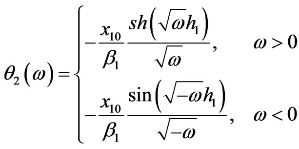
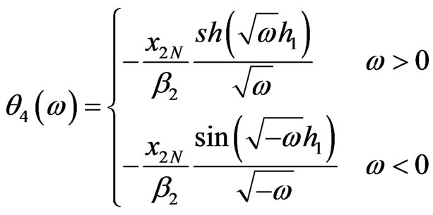
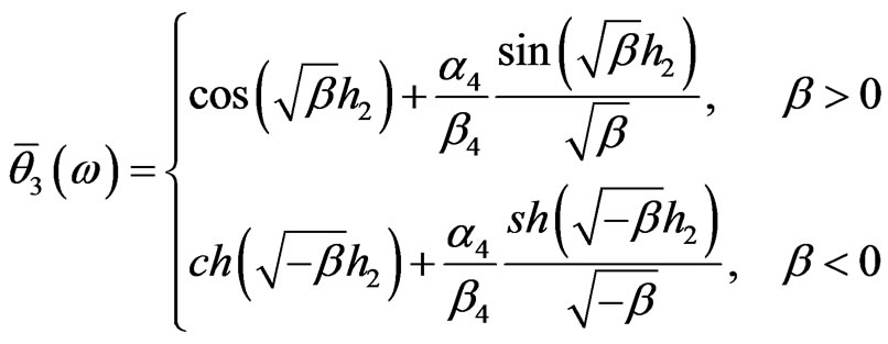
In the same way, as before, one can construct the best difference boundary conditions for . We omit the evaluation and present only the final results:
 , when
  (4.6a)
 when
when  (4.6b)
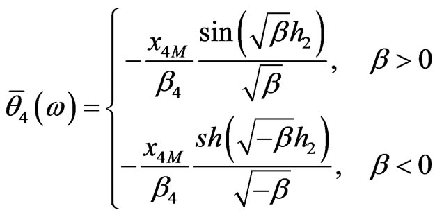
and
 when
when  (4.7a)
 when
when  (4.7b)
where  are defined by
 (4.8a)
 (4.8b)
and
 (4.9a)
 (4.9b)
5. Method for Solution of Finite-Difference Equations
In this section we consider a method for solving the finite-difference Equations (3.7). For this purpose we rewrite it in the from
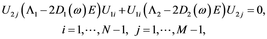 (5.1)
(5.1)
in which we have used (3.11) From this it is clear, that Equation (5.1) will be fulfilled if we choose  and
and  such that
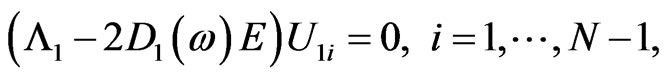 (5.2a)
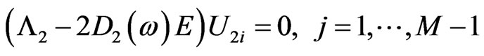 (5.2b)
The last weakly coupled system of Equation (5.2) is splitted into two equations with corresponding boundary conditions. First, we consider the Equation (5.2a) subject to boundary conditions (4.2) and (4.4).
According to (2.1), (2.2) and (2.3) the function  will be defermined within an arbitrary multiplicative constant. Therefore the three-point finite-difference Equation (5.2a) can be solved by shooting method starting with
 ,
,  and
and  which are required to be known. Thanks to (4.2) it is possible to find
  or
or  depending on the
 . For example, if
  then
then  is determined by (4.2a) and
  and ω to be chosen arbitrary. Otherwise,
  is determined by (4.2b) and
  and ω to be chosen arbitrary.
Note, that when  one of the boundary conditions (2.5), (2.6) is assumed to be homogeneous. For Laplace’s equation we always can leads to equation with homogeneous boundary conditions by change of variables. The exact value of parameter ω must satisfy
 (5.3)
(5.3)
where , for examples, when
  defined by
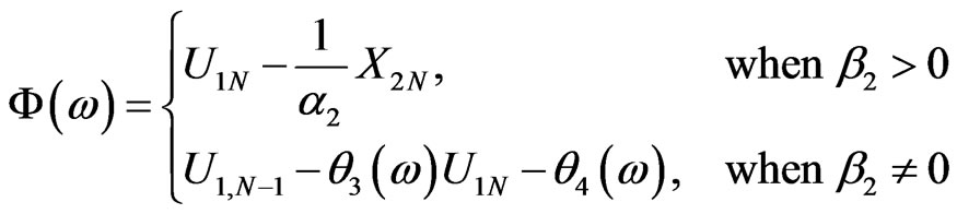 (5.4)
(5.4)
The nonlinear Equation (5.3) can be solved by Newton’s method:
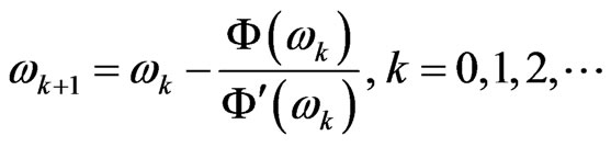 (5.5)
(5.5)
The value  in the dominator of (5.5) is found by differentiating the Equation (5.4) and (5.2a) with respect to ω. The iteration process (5.5) is terminated by criterion
 (5.6)
(5.6)
where  is a reassigned accuracy.
If the evaluation of  causes some difficulty we can use secant method instead of Newton’s ones. After finding ω the three-point difference equations (5.2b) with boundary conditions (4.6), (4.7) can be solved by elimination method.
6. Numerical Results
We have tested the efficiency and accuracy of finitedifference scheme (3.7) on the several examples.
Example 1.

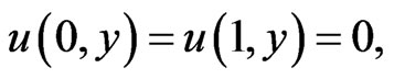
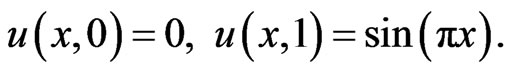
with boundary condition

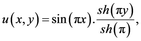
The exact solution is given by
In Table 1 we present the computed values of  (exact values of
  present in brackets) for N = 5 and M = 4. In order to use secant method we need two first approximations
  and
and  to ω. The iteration was terminated by criterion (5.6) with
 .
.
Example 2.
with boundary condition
The exact solution is given by
In Table 2 we present the computed values of
 (exact values of
  present in brackets) for N = 6 and M = 6. In order to use secant method we need two first approximations
  and
and  to ω. In this example choose
  and
and . The exact value of ω is
  The convergence of
  was tabulated in Table 3. The iteration was terminated by criterion (5.6) with
 .
.
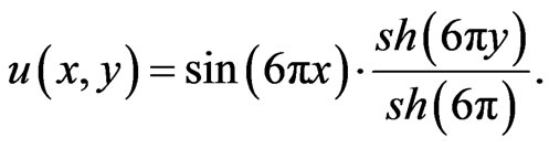
Example 3.
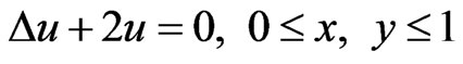
with boundary condition

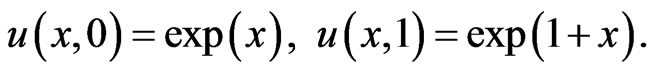
The exact solution is given by
In Table 4 we present the computed values of
 (exact values of
  present in brackets) for N = 6 and M = 4. In order to use secant
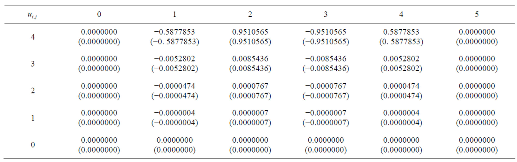
Table 1. Computed values of  for N = 5 and M = 4.
Table 2. Computed values of  for N = 6 and M = 6.

Table 3. The convergence of .
.
Table 4. Computed values of  for N = 6 and M = 4.
Table 5. The convergence of .
.
method we need two first approximations  and
and  to ω. In this example we were choose
  and
and . The exact value of ω is
 . The convergence of
  was tabulated in Table 5. The iteration was terminated by criterion (5.6) with ε = 10−7.
REFERENCES
- R. P. Agarwal, “Difference Equations and Inequalities: Theory, Methods and Applications,” 2nd Edition, CRC Press, Boca Raton, 2000.
- R. E. Mickens, “Nonstandard Finite Difference Models of Differential Equations,” World Scientific, Singapore, 1994.
- A. A. Samarskii, “Theory of Difference Equations,” 1977.
- B. Batgerel and T. Zhanlav, “An Exact Finite-Difference Scheme for Sturm-Liouville Problems,” South Carolina, Vol. 1, No. 120, 1996, pp. 8-15.